Category: Easy

  • ML0049 Logistic Regression II

    Please compare Logistic Regression and Neural Networks.

    Answer

    Logistic Regression is a straightforward, linear model suitable for linearly separable data and offers good interpretability. In contrast, Neural Networks are powerful, non-linear models capable of capturing intricate patterns in large datasets, often at the expense of interpretability and higher computational demands.

    The table below compares Logistic Regression and Neural Networks in more detail.


    Login to view more content
  • ML0048 Logistic Regression

    Can you explain logistic regression and how it contrasts with linear regression?

    Answer

    Logistic regression maps inputs to a probability space for classification, while linear regression estimates continuous outcomes through a direct linear relationship.

    Logistic regression model estimates the probability that a binary outcome (y = 1) occurs, given an input vector (x)
    \Pr(y=1 \mid \mathbf{x}) = \frac{1}{1 + e^{-(\mathbf{w}^{\top}\mathbf{x} + b)}}
    Where:
    \mathbf{x} is the input feature vector,
    \mathbf{w} is the weight vector, and
    b is the bias term.

    Logistic Regression vs. Linear Regression:
    Linear Regression:
    Purpose: Predicts a continuous output (e.g., price, height).
    Output: Real number (can be negative or >1).
    Assumes: Linearity between input features and output.

    Logistic Regression:
    Purpose: Predicts a probability for classification (e.g., spam or not).
    Output: Value between 0 and 1 using sigmoid function.
    Interpreted as: Probability of class membership.

    Here is a table comparing Logistic Regression with Linear Regression.


    Login to view more content
  • ML0047 Parameters

    What are the differences between parameters and hyperparameters?

    Answer

    Parameters are the values that a model learns from its training data, while hyperparameters are settings defined by the user that guide the training process and model architecture.

    Parameters:
    (1) Internal variables learned from data (e.g., weights and biases).
    (2) Adjusted during training using optimization algorithms.
    (3) Capture the model’s learned patterns and information.

    Hyperparameters:
    (1) External configurations set before training (e.g., learning rate, batch size, number of layers).
    (2) Remain fixed during training and are not updated by the learning process.
    (3) Influence how the model learns and its overall structure.


    Login to view more content
  • ML0046 Forward Propagation

    Please explain the process of Forward Propagation.

    Answer

    Forward propagation is when a neural network takes an input and generates a prediction. It involves systematically passing the input data through each layer of the network. A weighted sum of the inputs from the previous layer is calculated at each neuron, and then a nonlinear activation function is applied. This process is repeated layer by layer until the data reaches the output layer, where the final prediction is generated.

    Here is the process of Forward Propagation:
    (1) Input Layer: The network receives the raw input data.
    (2) Layer-wise Processing:
    Linear Combination: Each neuron calculates a weighted sum of its inputs and adds a bias.
    Non-linear Activation: The resulting value is passed through an activation function (e.g., ReLU, sigmoid, tanh) to introduce non-linearity.
    (3) Propagation Through Layers: The output from one layer becomes the input for the next layer, progressing through all hidden layers.
    (4) Output Generation: The final layer applies a function (like softmax for classification or a linear function for regression) to produce the network’s prediction.


    Login to view more content

  • ML0045 Multi-Layer Perceptron

    What is a Multi-Layer Perceptron (MLP)? How does it overcome Perceptron limitations?

    Answer

    A Multi-Layer Perceptron (MLP) is a feedforward neural network with one or more hidden layers between the input and output layers. Hidden layers in MLP use non-linear activation functions (like ReLU, sigmoid, or tanh) to model complex relationships. MLP can be used for classification, regression, and function approximation. MLP is trained using backpropagation, which adjusts the weights to minimize errors.

    Overcoming Limitations:
    (1) Learn non-linear: Unlike a single-layer perceptron that can only solve linearly separable problems, an MLP can learn non-linear decision boundaries, handling problems such as the XOR problem.
    (2) Universal Approximation: With enough neurons and layers, an MLP can approximate any continuous function, making it a powerful model for various applications.

    The plot below illustrates an example of a Multi-Layer Perceptron (MLP) applied to a classification problem.


    Login to view more content
  • ML0044 Perceptron

    Describe the Perceptron and its limitations.

    Answer

    The perceptron is a simple linear classifier that computes a weighted sum of input features, adds a bias, and applies a step function to produce a binary decision. The perceptron works well only for data sets that are linearly separable, where a straight line (or hyperplane in higher dimensions) can separate the classes.

    The perception output can be calculated by
     y = f(w^T x + b)
    Where:
     y is the predicted output (0 or 1)
     w is the weight vector
     x is the input vector
     b is the bias term
     f(\cdot) is the activation function (typically a step function)

    Below shows a perceptron diagram.

    Limitations for using perception:
    (1) Linearly Separable Data Only: Cannot solve problems like XOR, which are not linearly separable.
    (2) Single-Layer Only: Cannot model complex or non-linear patterns.
    (3) No Probabilistic Output: Outputs only binary values, not confidence or probabilities.


    Login to view more content
  • ML0043 Feature Scaling

    Walk me through the rationale behind Feature Scaling in machine learning.

    Answer

    Feature scaling is a fundamental data preprocessing step that normalizes or standardizes the range of numerical features. It is essential for many machine learning algorithms to ensure that all features contribute equally to the model, leading to faster convergence, improved accuracy, and better overall model performance, especially for algorithms sensitive to the magnitude of feature values or those based on distance calculations.

    Definition: Process of normalizing or standardizing input features so they’re on a similar scale.
    Why Needed: Many ML models (e.g., SVM, KNN) are sensitive to feature magnitude. Prevents dominant features from overpowering others due to scale.

    Common Methods:
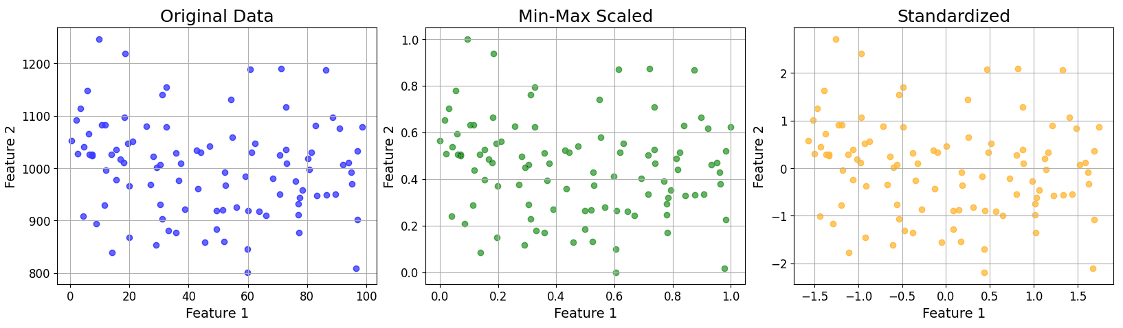
    Min-Max Scaling: Scales features to a range (usually [0, 1]).
    \mbox \quad X_{\text{normalized}} = \frac{X - X_{\text{min}}}{X_{\text{max}} - X_{\text{min}}}
    Where:
     X represents the original value of the feature.
     X_{\text{min}} represents the minimum value of the feature in the dataset.
     X_{\text{max}} represents the maximum value of the feature in the dataset.

    Standardization (Z-score Normalization, centers data to mean 0, standard deviation to 1):
    \mbox \quad X_{\text{standardized}} = \frac{X - \mu}{\sigma}
    Where:
     X represents the original value of the feature.
     \mu represents the mean of the feature in the dataset.
     \sigma represents the standard deviation of the feature in the dataset.

    Below shows an example plot for original, min-max scaled, and standardized data.


    Login to view more content

  • ML0042 Early Stopping

    What is Early Stopping? How is it implemented?

    Answer

    Early Stopping is a regularization technique used to halt training when a model’s performance on a validation set stops improving, thus avoiding overfitting. It monitors metrics like validation loss or validation accuracy and stops after a defined number of stagnant epochs (patience). This ensures efficient training and better generalization.

    Implementation:
    Split data into training and validation sets.
    After each epoch, evaluate on the validation set.
    If performance improves, save the model and reset the patience counter.
    If no improvement, counter add one; if the counter reaches the patience epochs, stop training.
    Restore best weights after stopping, load the model weights from the epoch that yielded the best validation performance.

    Below is one example loss plot when using early stop.


    Login to view more content
  • ML0041 Concept of NN

    Please explain the concept of a Neural Network.

    Answer

    A neural network (NN) is a machine learning model composed of layers of interconnected neurons. It learns patterns in data by adjusting weights through training, enabling it to perform tasks like classification, regression, and more.

    (1) Inspired by Biology: Neural networks are computer systems modeled after the human brain’s network of neurons.
    (2) Layered Structure: Neural networks consist of an input layer, one or more hidden layers, and an output layer.
    (3) Neurons and Activation: Each neuron performs a weighted sum of its inputs, adds a bias, and applies an activation function to produce an output. Weights and Biases are learnable parameters adjusted during training. Activation Functions can introduce non-linearity (e.g., ReLU, Sigmoid).
    (4) Learning Process: Neural networks learn by adjusting the weights and biases through training algorithms such as backpropagation, minimizing errors between predictions and actual results.
    (5) Versatility in Applications: Neural networks can identify complex patterns, making them suitable for tasks like image recognition, natural language processing, and data classification.

    Below shows an example of an NN.


    Login to view more content
  • ML0040 Bias and Variance

    Can you explain the bias-variance tradeoff?

    Answer

    Bias:
    Error due to overly simplified assumptions in the model.
    High bias may lead to underfitting, where the model misses key patterns in the data.

    Variance:
    Error due to high sensitivity to variations in the training data.
    High variance may result in overfitting, where the model captures noise and underlying patterns.

    Bias-Variance Tradeoff:
    Increasing model complexity typically decreases bias but increases variance, while a simpler model increases bias but decreases variance.
    The goal is to balance both to minimize the total error on unseen data.

    The bias-variance tradeoff illustrates that there’s a delicate balance to strike when building a machine learning model. A simpler model tends to have high bias and low variance, underfitting the data. A more complex model tends to have low bias and high variance, overfitting the data. The goal is to find the right level of model complexity to minimize the total prediction error, which is the sum of squared bias, variance, and irreducible error.

    The example below shows scenarios of high bias (underfitting), high variance (overfitting), and a good balance.


    Login to view more content