Interview for Machine Learning

Category: Medium

ML0064 Random Forest II
Please explain the benefits and drawbacks of random forest.
Answer
Random Forest is a powerful ensemble method that reduces overfitting and improves predictive accuracy by combining many decision trees. However, it trades interpretability and computational efficiency for these benefits and may require careful tuning when dealing with large, imbalanced, or sparse datasets.
Benefits of random forest:
(1) Reduces Overfitting: Aggregating many trees lowers variance.
(2) Robust to Noise and Outliers: Less sensitive to anomalous data.
(3) Handles High Dimensionality: Works well with many input features.
(4) Estimates Feature Importance: Helps identify influential variables.
(5) Built-in Bagging: Bootstrap sampling improves generalization.
Drawbacks of random forest:
(1) Less Interpretability: Hard to visualize or explain compared to a single decision tree.
(2) Computational Cost: Training and prediction can be slower with many trees.
(3) Memory Usage: Large forests can consume significant resources.
(4) Biased with Imbalanced Data: Class imbalance can lead to biased predictions.
(5) Not Always Optimal for Sparse Data: May underperform compared to other algorithms on very sparse datasets.
The example below demonstrates that the random forest sometimes underperforms on the imbalanced dataset.
Login to view more content
July 8, 2025
ML0060 K Selection in K-Means
How to select K in K-Means?
Answer
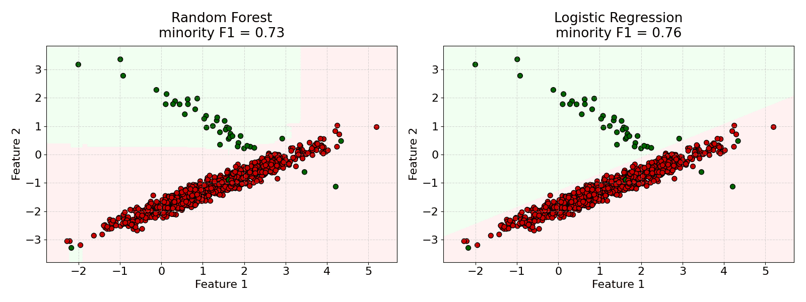
To select the optimal number of clusters $K$ in K-Means, use the visual plot like the elbow method, quantitative metrics like the silhouette score, or statistical methods like the gap statistic. These help balance model fit and generalization without overfitting.
Elbow Method:
(1) Plot the within-cluster sum of squares (WCSS) vs. $K$ .
(2) Choose the “elbow” point where the rate of improvement slows.
WCSS can be calculated using the following equation:
$\text{WCSS}(K) = \sum_{k=1}^{K} \sum_{x_i \in C_k} |x_i - \mu_k|^2$
Where:
$C_k$ is cluster $k$ ,
$\mu_k$ is its centroid.
Here is one plot example to demonstrate the location of the elbow point.
Silhouette Score:
The silhouette score measures how well each point lies within its cluster. It ranges from -1 (wrong clustering) to 1 (well-clustered).
(1) Calculate the average silhouette score for different $K$ values.
(2) Choose the $K$ that yields the highest average silhouette score.
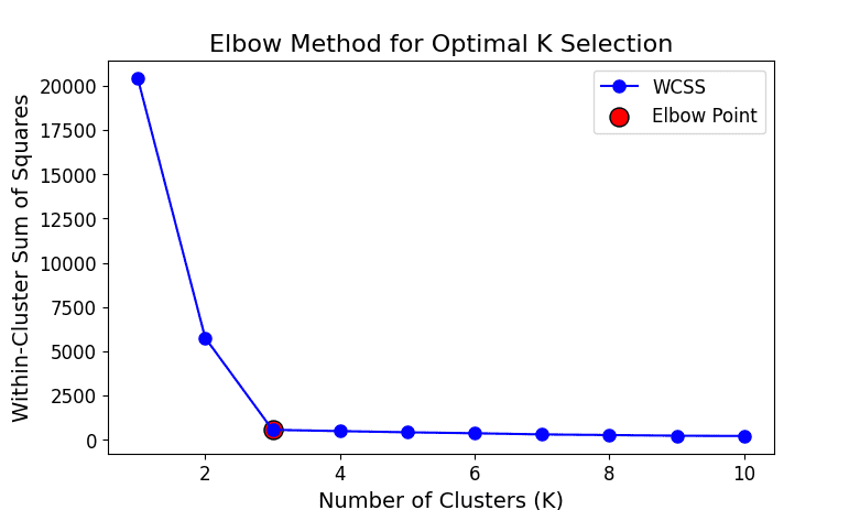
Silhouette coefficient for point $i$ can be calculated by the following equation.
$s(i) = \frac{b(i) - a(i)}{\max(a(i), b(i))}$
Where:
$a(i)$ = intra-cluster distance,
$b(i)$ = nearest-cluster distance.
Gap Statistic:
(1) Compares clustering against a random reference distribution.
(2) Choose $K$ that maximizes the gap between observed and expected WCSS.
Login to view more content
June 14, 2025
ML0058 K-means++
Please explain how K-means++ works.
Answer
K-means++ is an improved way to initialize centroids in K-means. K-means++ selects initial centroids one by one using a weighted probability based on squared distances from already chosen centroids. This spreads out the centroids more effectively, reducing the chances of poor clustering and helping the algorithm converge faster and more reliably.
K-means++ Steps:
(1) Choose the first centroid $\mu_1$ uniformly at random from the dataset.
(2) For each point $x_i$ , compute its squared distance to the nearest chosen centroid:
$D(x_i)^2 = \min_{1 \le j \le m} |x_i - \mu_j|^2$
Where:
$\mu_j$ is one of the already chosen centroids.
(3) Choose the next centroid $\mu_{m+1}$ with probability:
$P(x_i) = \frac{D(x_i)^2}{\sum_j D(x_j)^2}$
Where:
$D(x_i)^2$ is the squared distance from point $x_i$ to its nearest already chosen centroid.
$\sum_j D(x_j)^2$ is the sum of minimum squared distances from all data points to their nearest chosen centroid.
(4) Repeat until $K$ centroids are chosen.
(5) Then proceed with standard K-means clustering.
Below shows an example for K-means++ clustering.
Login to view more content
June 12, 2025
ML0056 K Selection in KNN
In the context of designing a K-Nearest Neighbors (KNN) model, can you explain your approach to selecting the value of K?
Answer
Selecting the optimal value for ‘K’ in a K-Nearest Neighbors (KNN) model is crucial as it significantly impacts the model’s performance.
(1) Bias-Variance Tradeoff: The choice of K involves balancing bias and variance.
A small $K$ (e.g., 1) leads to low bias and high variance, often resulting in overfitting.
A large $K$ increases bias but reduces variance, potentially underfitting the data.
(2) Use Odd Values for Classification: In binary classification, odd $K$ avoids ties.
(3) Cross-Validation Combined with Grid Search: Use k-fold cross-validation to evaluate performance across multiple values of $K$ , and select the one that minimizes the validation error.
Cross-Validation Error can be calculated by the below equation.
$CV(K) = \frac{1}{N}\sum_{i=1}^{N} \ell\big(y_i, \hat{y}_i(K)\big)$
Where:
$y_i$ is the actual outcome for the i‑th instance.
$\hat{y}_i(K)$ represents the predicted value using $K$ neighbors.
$N$ is the total number of validation samples.
$\ell$ is a loss function.
(4) Domain Knowledge: In some cases, prior knowledge for the data distribution can help select a reasonable range of $K$ .
The example below apply k-fold cross-validation with grid search for K selection in one KNN regression task.
Login to view more content
June 12, 2025
ML0052 Non-Linear SVM
Can you explain the concept of a non-linear Support Vector Machine (SVM)?
Answer
A non-linear SVM allows classification of data that isn’t linearly separable by using a kernel function to project the data into a higher-dimensional space implicitly. This approach, known as the kernel trick, provides flexibility in handling complex datasets while maintaining computational efficiency. The choice of kernel, such as RBF, polynomial, or sigmoid, can greatly influence the performance and adaptability of the model.
Kernel Trick: Converts input data into a higher-dimensional space where a linear separation is possible, even if the original data is non-linearly separable.
Common Kernels:
Polynomial Kernel:
Uses polynomial functions of the input features to capture non-linear patterns in the data.
$K(\mathbf{x}_i, \mathbf{x}_j) = (\gamma \mathbf{x}_i^\top \mathbf{x}_j + c)^d$
Where:
$\mathbf{x}_i, \mathbf{x}_j$ are input vectors.
$\gamma$ controls the scale of the inner product.
$c$ is a constant that controls the influence of higher-order terms.
$d$ is the degree of the polynomial.
Radial Basis Function (RBF) Kernel:
Measures local similarity based on the Euclidean distance between points; nearby points have higher similarity.
$K(\mathbf{x}_i, \mathbf{x}_j) = \exp\left(-\gamma \|\mathbf{x}_i - \mathbf{x}_j\|^2\right)$
Where:
$\mathbf{x}_i, \mathbf{x}_j$ are input vectors.
$\|\mathbf{x}_i - \mathbf{x}_j\|^2$ is the squared Euclidean distance between the vectors.
$\gamma$ controls the scale of the inner product.
$\sigma$ is a parameter that controls the width of the Gaussian (spread).
Sigmoid Kernel:
Imitates neural activation by applying a tanh function to the dot product of inputs, introducing non-linearity.
$K(\mathbf{x}_i, \mathbf{x}_j) = \tanh(\gamma \mathbf{x}_i^\top \mathbf{x}_j + c)$
Where:
$\mathbf{x}_i, \mathbf{x}_j$ are input vectors.
$\gamma$ controls the scale of the inner product.
$c$ is a bias term.
Objective: Determine an optimal hyperplane in the transformed space that maximizes the margin between classes, effectively improving classification performance.
$\max_{\boldsymbol{\alpha}} \sum_{i=1}^{n} \alpha_i - \frac{1}{2} \sum_{i=1}^{n} \sum_{j=1}^{n} \alpha_i \alpha_j y_i y_j K(\mathbf{x}_i, \mathbf{x}_j)$
The example below compares a Linear Support Vector Machine with a Non-Linear Support Vector Machine.
Login to view more content
June 11, 2025
ML0050 Logistic Regression III
Why is Mean Squared Error (L2 Loss) an unsuitable loss function for logistic regression compared to cross-entropy?
Answer
Mean Squared Error (MSE) is unsuitable for logistic regression primarily because, when combined with the sigmoid function, it can lead to a non-convex loss landscape, making optimization harder and increasing the risk of poor convergence. Additionally, it provides weaker gradients when predictions are confidently incorrect, slowing down learning. Cross-entropy loss is better suited as it aligns with the Bernoulli distribution assumption, produces stronger gradients, and leads to a well-behaved convex loss for a single neuron binary classification setting.
(1) Wrong Assumption: MSE assumes a Gaussian distribution of errors, while logistic regression assumes a Bernoulli (binary) distribution.
(2) Non-convex Optimization: MSE with sigmoid can create a non-convex loss surface, making optimization harder and less stable.
(3) Gradient Issues: MSE leads to smaller gradients for confident wrong predictions, slowing down learning compared to cross-entropy.
(4) Interpretation: Cross-entropy directly compares predicted probabilities to true labels, which is more appropriate for classification.
The figure below shows the non-convex loss surface when MSE is used for logistic regression.
Login to view more content
June 10, 2025
ML0033 All Zeros Init
How does initializing all weights and biases to zero affect a neural network’s training?
Answer
Initializing all weights and biases to zero forces neurons to behave identically, leading to uniform gradient updates that prevent the network from learning diverse representations.
(1) Symmetry Problem: Neurons receive identical gradients, causing them to learn the same features rather than developing distinct representations.
(2) Limited Representational Capacity: The network cannot capture complex, varied patterns because all neurons behave identically.
(3) Slow/No Convergence: The lack of Representational Capacity further makes it difficult for the model to update to the optimal weights.
(4) Zero Output (Potentially): For some activation functions (like ReLu), with zero weights and biases, the initial output of every neuron will be zero. This can lead to zero gradients in the subsequent layers, halting the learning process entirely.
Here is an example comparing initializing all weights and biases to zero vs random initialization for a binary classification problem.
Login to view more content
May 6, 2025
ML0029 Tanh
What are the advantages and disadvantages of using the tanh activation function?
Answer
In machine learning, the hyperbolic tangent (tanh) activation function is defined as
$\mbox{tanh}(x) = \frac{e^{x} - e^{-x}}{e^{x} + e^{-x}}$
This function transforms input values into a range between -1 and 1, helping with faster convergence in neural networks.
Advantages:
(1) Zero-centered outputs: Unlike sigmoid, which outputs values between 0 and 1, tanh produces values between -1 and 1, making optimization easier and reducing bias in gradient updates.
(2) Smooth and Differentiable: The function is infinitely differentiable, supporting stable gradient‑based methods.
Disadvantages:
(1) Vanishing gradient problem: For very large or very small input values, the derivative of tanh approaches zero, leading to slow weight updates and potentially hindering deep network training.
(2) Computationally expensive: Compared to ReLU, tanh requires exponentially complex calculations, which may slow down model inference.
Login to view more content
April 17, 2025
ML0027 Leaky ReLU
What are the benefits of the Leaky ReLU activation function?
Answer
Leaky ReLU modifies the standard ReLU by allowing a small, non-zero gradient for negative inputs. Its formula is typically written as:
${\large \text{Leaky ReLU}(x) = x \text{ if } x \ge 0,\quad \alpha x \text{ if } x < 0}$
Advantages of Leaky ReLU:
1. Addresses the dying ReLU problem: By having a small non-zero slope for negative inputs, Leaky ReLU allows a small gradient to flow even when the neuron is not active in the positive region. This prevents neurons from getting stuck in a permanently inactive state and potentially helps them recover during training.
2. Retains the benefits of ReLU for positive inputs: Maintains the linearity and non-saturation for positive values, contributing to efficient computation and gradient propagation.
Login to view more content
April 12, 2025
ML0025 Exploding Gradient
What are the typical reasons for exploding gradient?
Answer
Exploding gradients occur when the gradients during backpropagation become excessively large. This leads to huge updates in the model’s weights, making the training process unstable and potentially causing the model to diverge instead of converging.
Typical Reasons for Exploding Gradients:
1. Deep Architectures:
In very deep networks, repeatedly multiplying gradients (especially when derivatives are >1) can cause them to grow exponentially
2. Large Learning Rates:
When the learning rate is set too high, even moderately large gradients can result in weight updates that overshoot the optimum by a significant margin, compounding the instability.
3. Improper Weight Initialization:
If weights are initialized to values that are too high, activations and their corresponding derivatives can be disproportionately large. This imbalance not only disrupts the symmetry in learning but can also contribute to the accumulation of large gradient values.
4. Activation Functions with Derivatives Greater Than 1:
Some activation functions or their operating regimes can have derivatives greater than 1. Repeated multiplication of these large derivatives during backpropagation can lead to exponential growth of the gradients.
Scaled Exponential Linear Unit (SELU). For positive inputs, the SELU is defined as:
${\large \text{SELU}(x) = \lambda x,\quad \text{for } x>0}$
In the typical configuration for self-normalizing neural networks, the parameter ${\large\lambda}$ is set to approximately 1.0507 (greater than 1). This means in the positive regime, each layer effectively amplifies the gradient by a factor of ${\large\lambda}$ , which, when compounded over many layers, can contribute to exploding gradients if not properly managed.
Login to view more content
April 4, 2025