Can you explain the concept of a non-linear Support Vector Machine (SVM)?
Answer
A non-linear SVM allows classification of data that isn’t linearly separable by using a kernel function to project the data into a higher-dimensional space implicitly. This approach, known as the kernel trick, provides flexibility in handling complex datasets while maintaining computational efficiency. The choice of kernel, such as RBF, polynomial, or sigmoid, can greatly influence the performance and adaptability of the model.
Kernel Trick: Converts input data into a higher-dimensional space where a linear separation is possible, even if the original data is non-linearly separable.
Common Kernels:
Polynomial Kernel:
Uses polynomial functions of the input features to capture non-linear patterns in the data.

Where: are input vectors.
 controls the scale of the inner product.
 is a constant that controls the influence of higher-order terms.
 is the degree of the polynomial.
Radial Basis Function (RBF) Kernel:
Measures local similarity based on the Euclidean distance between points; nearby points have higher similarity.
Where: are input vectors. is the squared Euclidean distance between the vectors. controls the scale of the inner product.
 is a parameter that controls the width of the Gaussian (spread).
Sigmoid Kernel:
Imitates neural activation by applying a tanh function to the dot product of inputs, introducing non-linearity.
Where: are input vectors. controls the scale of the inner product. is a bias term.
Objective: Determine an optimal hyperplane in the transformed space that maximizes the margin between classes, effectively improving classification performance.

The example below compares a Linear Support Vector Machine with a Non-Linear Support Vector Machine.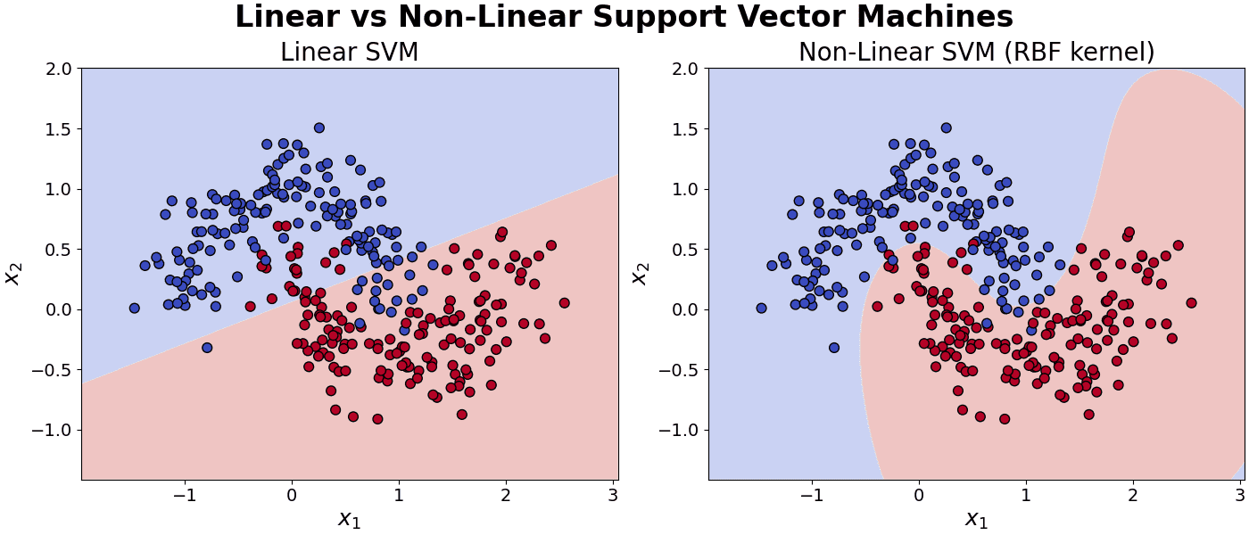
Leave a Reply