
How does XGBoost improve upon the classical gradient-boosted decision tree algorithm?
Answer
XGBoost keeps the sequential additive recipe of classical gradient boosting but upgrades it on three axes. First, optimization: it fits each tree with a second-order Taylor approximation of the loss, using both gradients and Hessians, so leaf weights and split gains are Newton-style steps instead of plain gradient steps. Second, regularization: the objective explicitly penalizes the number of leaves and the squared leaf weights, which prunes weak splits analytically. Third, systems: sparsity-aware split finding, a weighted quantile sketch for approximate splits, and cache-aware block layouts let it scale to billions of examples. The result dominated competitions: 17 of the 29 winning solutions published on Kaggle’s blog in 2015 used XGBoost.
(1) Second-Order Optimization: gradients alone say which way is downhill; Hessians say how curved the surface is, so XGBoost computes closed-form optimal leaf weights and exact split gains per candidate split.
(2) Regularized Objective: the penalty on leaf count and weight magnitude means a split must beat an explicit complexity cost to survive, a built-in analogue of pruning that classical GBDT lacks.
(3) Systems Engineering: default directions for missing values, approximate split proposals from weighted quantiles, and out-of-core cache-aware blocks deliver the reported 10x-plus speedups that made it the industry default.
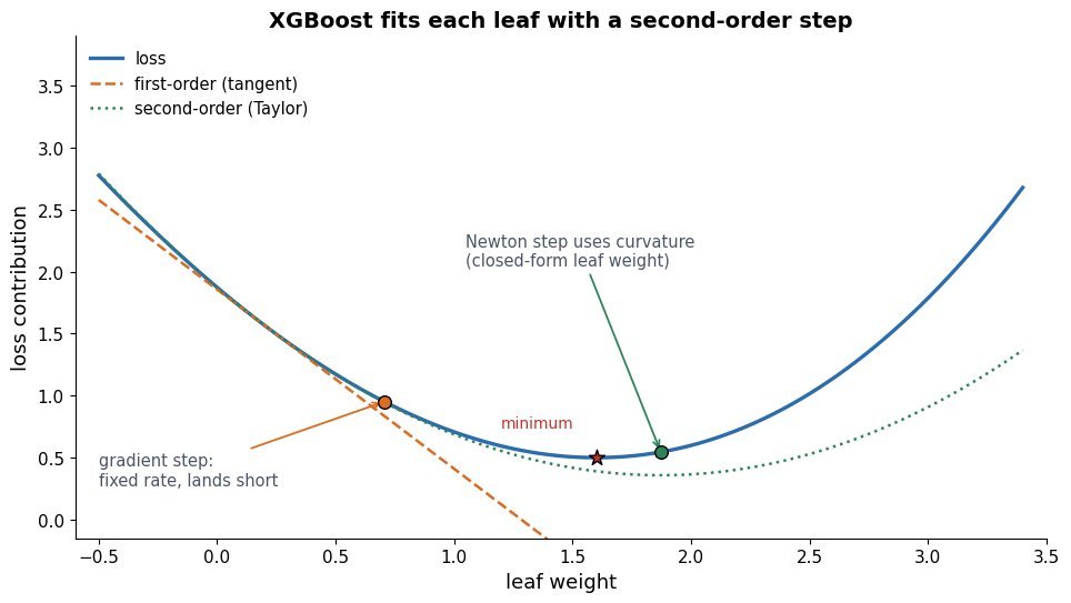
Figure 1: Why the Hessian helps: a first-order step moves along the tangent and misses the valley; a second-order step accounts for curvature (dashed parabola) and lands near the minimizer, which is what closed-form leaf weights do for every leaf.
The second-order view also explains where the regularization bites. Once you collect all examples routed to a leaf, the objective contribution of that leaf is a one-dimensional quadratic in its weight, whose closed-form minimizer shrinks toward zero as the penalty grows. Splits are scored by how much they reduce the total objective including the per-leaf cost, so a split that adds two leaves must overcome an explicit gamma toll twice. Classical GBDT instead fits trees to raw gradients and controls complexity only indirectly through depth caps and shrinkage.
Mathematical Formulation:


Where:
 and are the first and second derivatives of the per-example loss at the current prediction; is the new tree.
- is the regularizer: charges per leaf ( leaves) and penalizes squared leaf weights .
- are the sums of over the examples routed to leaf , and is the closed-form optimal leaf weight; larger shrinks every leaf toward zero.
 and
 are the first and second derivatives of the per-example loss at the current prediction;
 is the new tree.
 is the regularizer:
 charges per leaf (
 leaves) and
 penalizes squared leaf weights
 .
 are the sums of
 over the examples routed to leaf
 , and
 is the closed-form optimal leaf weight; larger
| Aspect | Classical GBDT | XGBoost |
|---|---|---|
| Loss Information | First-order gradients (residuals) | Gradients + Hessians (second-order Taylor) |
| Regularization | Indirect: depth caps, shrinkage, subsampling | Explicit: gamma on leaf count, lambda on leaf weights |
| Split Finding | Exact scan or basic histograms | Weighted quantile sketch + sparsity-aware defaults |
| Scale | In-memory, single machine | Cache-aware blocks, out-of-core, distributed |
| Track Record | Strong but slow at scale | 17 of 29 Kaggle 2015 winning solutions; every KDDCup 2015 top-10 team |
Leave a Reply