
How does DBSCAN work, and what advantages does it have over k-means for clustering tasks like geospatial stop detection?
Answer
DBSCAN is a density-based clustering algorithm: it groups points that are packed closely together and labels isolated points as noise, all without being told how many clusters to find. For each point it counts how many points fall within a radius eps; any point whose eps-neighborhood holds at least min_samples points (counting itself) is a core point, and clusters grow by linking core points whose neighborhoods overlap, then attaching their non-core neighbors. K-means, by contrast, requires you to specify K upfront and partitions data into Voronoi cells around centroids, which forces spherical clusters and assigns every point somewhere even if it is an outlier. In geospatial applications, DBSCAN is used to cluster raw GPS pings into “stops” because the density-based approach naturally absorbs GPS jitter and ignores transient traffic halts without needing a predefined polygon count.
(1) Density-Connected Expansion: a cluster is the maximal set of density-reachable points from a core point; points with fewer than min_samples neighbors but inside a core’s eps-radius become border points, and points reachable from no core become noise.
(2) No K and Arbitrary Shapes: DBSCAN discovers the cluster count from the data and follows winding, non-convex boundaries, which k-means cannot do because its Voronoi partition assumes spherical, similarly sized groups.
(3) Production Pattern: geospatial pipelines chain DBSCAN then SVM on GPS streams for foot-traffic analysis, and embedding-based clustering pairs UMAP with HDBSCAN (hierarchical DBSCAN) for recursive clustering because it handles varying densities and auto-selects stable clusters without an eps parameter.
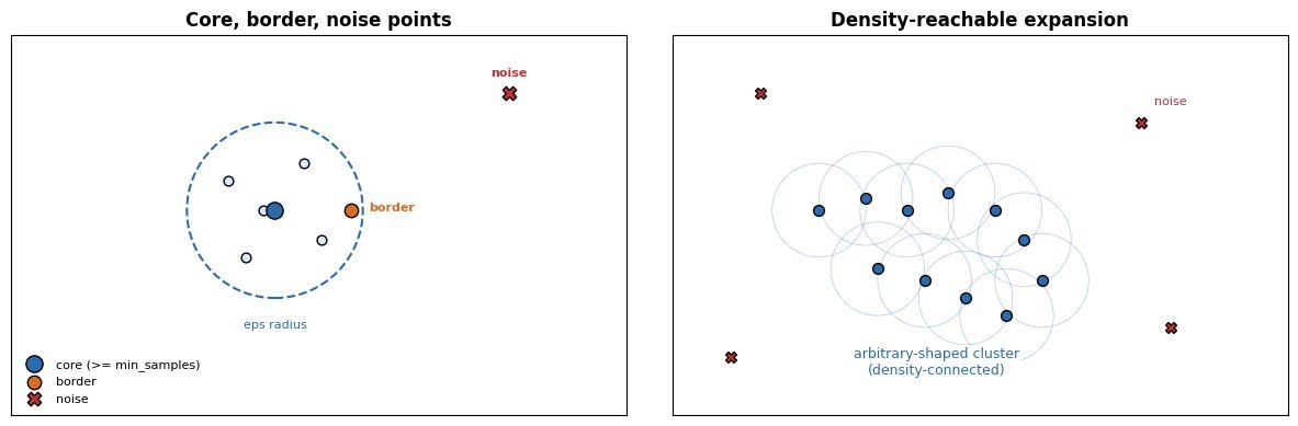
Figure 1: DBSCAN mechanics: a core point has at least min_samples neighbors inside the eps-radius circle; clusters expand by chaining overlapping core neighborhoods, border points attach to one cluster, and isolated points become noise.
The practical trade-off is parameter sensitivity and density variation. DBSCAN’s eps must be tuned to the data’s scale, and a single global eps struggles when clusters have different densities, which is why HDBSCAN extends DBSCAN into a hierarchy and extracts stable clusters at varying density levels. K-means is cheaper at scale (each iteration is O(nKd) and embarrassingly parallel) and wins when clusters are genuinely spherical and K is known, as in vector quantization for image compression. DBSCAN’s neighborhood queries cost O(n log n) with a spatial index but degrade to O(n^2) in high dimensions where indexing breaks down, so production pipelines reduce dimensionality with UMAP first.

Figure 2: On a non-convex two-moon dataset, k-means imposes a linear Voronoi cut that slices through both moons, while DBSCAN follows the curved density ridges and marks sparse-gap points as noise.
Mathematical Formulation:


Where:
 is the eps-neighborhood of point
  in dataset
  , and
, and  is typically Euclidean distance.
- A point is core when its neighborhood contains at least min_samples points; border points are in a core’s neighborhood but are not core themselves; noise points are in no core’s neighborhood.
- A cluster
 is the maximal set of points density-reachable from a core point via a chain of overlapping core neighborhoods; this transitive closure is what lets DBSCAN trace arbitrary shapes.
 is the eps-neighborhood of point
  in dataset
  , and
, and  is typically Euclidean distance.
 is the maximal set of points density-reachable from a core point via a chain of overlapping core neighborhoods; this transitive closure is what lets DBSCAN trace arbitrary shapes.
| Property | DBSCAN | k-means |
|---|---|---|
| Cluster Count | Discovered from density; no K needed | Must specify K upfront |
| Cluster Shape | Arbitrary, density-connected | Spherical Voronoi cells |
| Outliers | Labeled as noise explicitly | Force-assigned to nearest centroid |
| Parameters | eps, min_samples | K, initialization |
| Scalability | O(n log n) with spatial index; O(n^2) worst case | O(nK) per iteration, parallelizable |
| Weakness | Single eps fails on varying densities (HDBSCAN fixes this) | Breaks on non-spherical or unequal-size clusters |
Leave a Reply