Tag: CNN

  • DL0023 Dilated Convolution

    What are dilated convolutions? When would you use them?

    Answer

    Dilated convolutions (also called atrous convolutions) insert gaps between the elements of a convolutional kernel: with dilation rate d, the kernel samples every d-th input position instead of adjacent ones. This expands the receptive field without adding parameters and without reducing spatial resolution, a combination that pooling cannot offer. A dilation rate of 1 is just a standard convolution.

    (1) Larger Receptive Field, Same Weights: A 3×3 kernel with dilation 2 covers a 5×5 area but still has only 9 weights.
    (2) Resolution Preserved: Unlike pooling, dilation grows the receptive field while keeping the output the same size as a standard convolution, which is critical for dense prediction.
    (3) Multi-Scale Context: Stacking or mixing dilation rates lets one network aggregate both fine local detail and broad context.

    One-dimensional comparison of a standard kernel-3 convolution sampling three consecutive inputs versus a dilation-3 convolution sampling positions 0, 3, and 6 for a receptive field of seven with the same three weights.

    Figure 1: Same 3 weights, wider view: dilation 3 spreads the taps across a receptive field of 7 instead of 3.

    Mathematical Formulation:
    y_{ij} = \sum_{a=1}^{k}\sum_{b=1}^{k} w_{ab}\; x_{i + d \cdot a,\; j + d \cdot b}
    k_{eff} = k + (k - 1)(d - 1)

    Where:

    • d is the dilation rate, the spacing between tapped positions (d = 1 is standard convolution).
    • k is the nominal kernel size; k_{eff} is the effective span of the dilated kernel (3×3 with d = 2 behaves like 5×5 with holes).
    • w_{ab} are the kernel weights; the parameter count is independent of d.

    In Two Dimensions: The same idea applies to images: the kernel’s taps spread over a checkerboard-like stencil, expanding the covered span from 3×3 to 5×5 at dilation 2 while the channel count and output resolution stay unchanged.

    Two ten-by-ten grids comparing a dense 3x3 standard convolution stencil against a sparse 3x3 dilation-2 stencil that spans a 5x5 region marked by a red dashed receptive-field box.

    Figure 2: Dilation 2 turns a 3×3 stencil into a 5×5 receptive field (red dashed box), still only 9 multiply-accumulates.

    When to Use Them: Any task needing large context at full resolution: semantic segmentation (DeepLab), audio generation (WaveNet models long-range temporal structure with exponentially growing dilation), and dense tasks like super-resolution or depth estimation.

    Progression of a single input point through three stacked dilation-2 layers showing the response spreading into a checkerboard pattern with gaps between covered cells.

    Figure 3: Gridding artifacts: stacking the same dilation leaves a checkerboard of unattended cells. Mitigate with hybrid dilation rates (e.g., 1, 2, 5) that overlap coverage.

    Login to view more content
  • DL0022 CNN Architecture

    Describe the typical architecture of a CNN.

    Answer

    A typical Convolutional Neural Network chains together a small set of repeating building blocks: the raw input passes through stacked convolution + activation layers that extract local features, interleaved with pooling layers that halve the spatial resolution, after which the feature maps are flattened (or globally pooled) and fed into fully connected layers ending in a softmax output for classification. Regularizers such as dropout and batch normalization are commonly inserted along the way.

    (1) Feature Extraction Front-End: Repeated conv → ReLU → pool blocks build hierarchical features while shrinking spatial size and growing channels.
    (2) Classification Head: Flattened features (or a GAP vector) feed fully connected layers that combine features into class scores.
    (3) Output Layer: Softmax for multi-class, sigmoid for binary/multi-label; optional dropout, batch norm, and skip connections stabilize training.

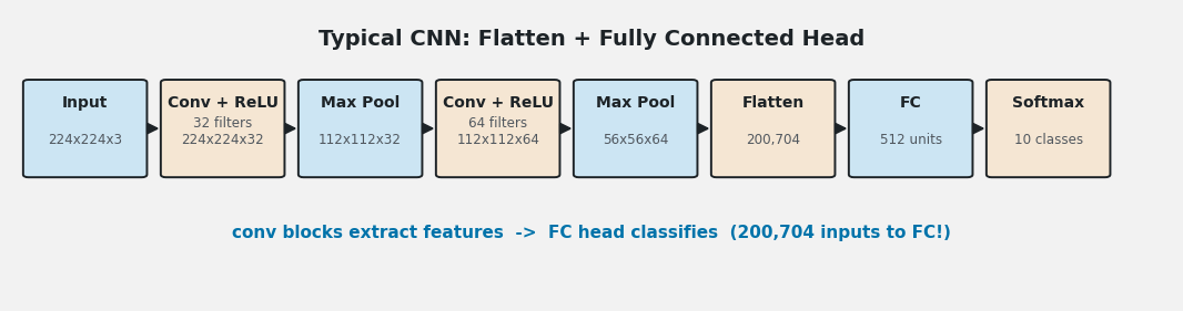
    Flow diagram of a typical CNN from a 224x224x3 input through two conv-ReLU-pool blocks, flattening to 200704 values, a 512-unit fully connected layer, and a 10-class softmax output.

    Figure 1: The canonical pipeline: spatial size shrinks (224 → 112 → 56) while channels grow (3 → 32 → 64), then a flatten + FC head classifies. Note the 200,704 values hitting the FC layer.

    Mathematical Formulation:
    W_{out} = \left\lfloor \frac{W_{in} - k + 2p}{s} \right\rfloor + 1
    P(y = i \mid z) = \frac{e^{z_i}}{\sum_{j=1}^{K} e^{z_j}}

    Where:

    • W_{in}, W_{out} are the input and output spatial sizes of a conv or pool layer; k is the kernel size, p the padding, s the stride.
    • z_i is the logit for class i; K is the number of classes; the softmax converts logits into a probability distribution.
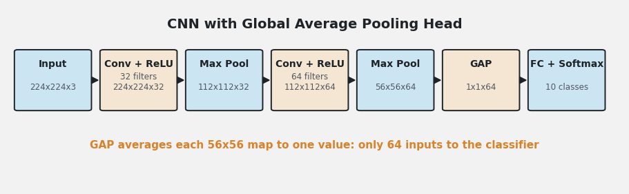
    Modern Variant: GAP Head: Many modern CNNs (ResNet, MobileNet) replace the flatten + large FC head with Global Average Pooling, which averages each feature map to a single number before a small classifier. This slashes parameters, removes the fixed-input constraint, and reduces overfitting.

    The same CNN front-end followed by a global average pooling layer producing 64 values that feed a small 10-class softmax classifier instead of a large fully connected layer.

    Figure 2: Swapping flatten for GAP shrinks the classifier input from 200,704 to 64 values, millions fewer parameters in the head.


    Login to view more content
  • DL0021 Feature Map

    What is the feature map in Convolutional Neural Networks?

    Answer

    A feature map is the output produced when one convolutional filter slides across its input: a 2D grid of activations whose values encode where and how strongly a specific pattern (an edge orientation, texture, or object part) appears at each spatial location. A convolutional layer applies many filters in parallel, so its output is a stack of feature maps, one per filter, forming the layer’s channels.

    (1) Output of One Filter: Each feature map is generated by a single filter convolving over the input; the layer output stacks one map per filter, so 64 filters produce 64 channels.
    (2) Location and Strength: A high activation at position (i, j) means the filter’s pattern (e.g., a vertical edge or a corner) is strongly present around that location.
    (3) Evolving Semantics with Depth: Early maps respond to edges and textures, middle maps to parts and shapes, and deep maps to whole objects with class-specific meaning.

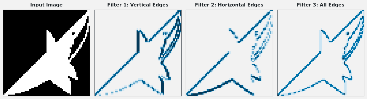
    An input silhouette and three feature maps produced by different filters showing vertical edges, horizontal edges, and all edges highlighted at their spatial locations.

    Figure 1: Three filters applied to the same input produce three different feature maps; each lights up where its own pattern (vertical, horizontal, or any edge) appears.

    Mathematical Formulation:
    y^{(c)}_{ij} = \sum_{a=1}^{k}\sum_{b=1}^{k}\sum_{d=1}^{C_{in}} w^{(c)}_{abd}\, x_{i+a,\, j+b,\, d} + b_c
    \text{output shape} = (H_{out},\ W_{out},\ C_{out}), \quad C_{out} = \text{number of filters}

    Where:

    • y^{(c)}_{ij} is the activation of feature map c at spatial position (i, j).
    • w^{(c)}_{abd} are the weights of filter c of size k \times k \times C_{in}; b_c is its bias.
    • x_{i+a,\, j+b,\, d} is the input activation; C_{in} and C_{out} are the input and output channel counts.
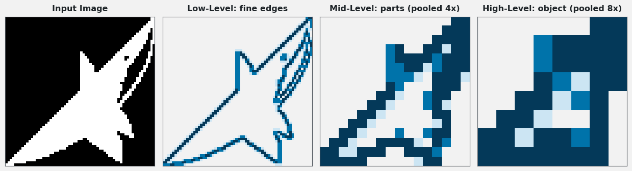
    Hierarchical Representation: As activations flow deeper, each new feature map is computed from the previous layer’s maps, so neurons see progressively larger receptive fields and combine simpler patterns into richer ones, the foundation of a CNN’s representational power.

    The same input shown with a fine low-level edge feature map, a coarser mid-level part feature map, and a blocky high-level object feature map illustrating the feature hierarchy.

    Figure 2: Depth turns fine edges into parts and finally into an object-level representation. Resolution drops while semantic content rises.


    Login to view more content
  • DL0020 CNN Parameter Sharing

    How do Convolutional Neural Networks achieve parameter sharing? Why is it beneficial?

    Answer

    CNNs share parameters by applying the same convolutional filter at every spatial location: a small kernel of learnable weights slides across the input, and its weights are reused to compute each output activation. This weight reuse means the network learns location-independent features with far fewer parameters than a fully connected layer, which improves generalization and compute efficiency.

    How Sharing Works:

    (1) Convolutional Filter: A small matrix of learnable weights (e.g., 3 \times 3) is defined per channel pair.
    (2) Sliding Window: The filter moves across the whole input feature map, position by position.
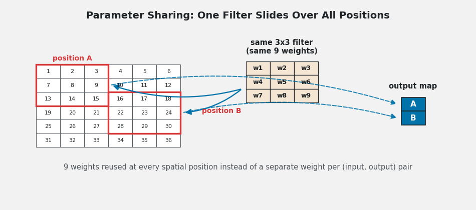
    (3) Weight Reuse: The identical weights are used at every position, so one filter detects its feature anywhere in the image.

    Diagram of one shared 3x3 filter with the same nine weights applied at two different positions of an input grid producing two output activations.

    Figure 1: The same 9 weights produce activations at position A and position B. No new parameters are added as the input grows.

    Why It Is Beneficial:

    (1) Reduced Parameters: A filter has k \times k \times C_{in} weights regardless of input resolution, versus one weight per (input, output) pair in an FC layer.
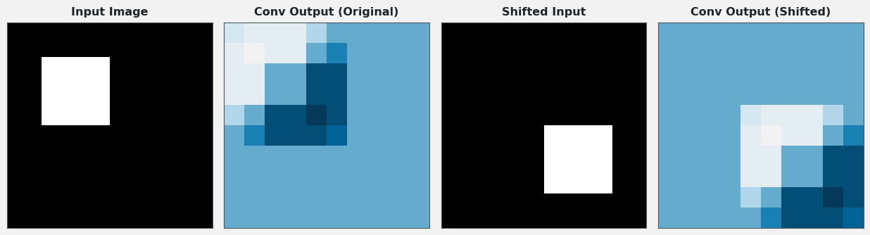
    (2) Translation Equivariance: A feature detected at one location is detected at any location; shifting the input shifts the output correspondingly.
    (3) Improved Generalization: Fewer parameters means less overfitting, especially on limited data.
    (4) Computational Efficiency: Fewer parameters mean fewer multiply-accumulates in both forward and backward passes, enabling deployment on resource-limited devices.

    Four panels showing an input image with a square, its convolution output, a shifted input, and the identically shifted convolution output demonstrating translation equivariance.

    Figure 2: Translation equivariance in action: shifting the input shifts the convolution output by the same amount, because the same shared filter processes every position.

    How Big Is the Saving? Sharing decouples the parameter count from the input resolution: growing the image grows the compute, not the weights. The contrast with a fully connected layer on the same input is dramatic.

    Log-scale bar chart comparing about 307 thousand parameters for a fully connected layer on a 32x32x3 input versus about 1.8 thousand for a shared 3x3 convolution.

    Figure 3: Flattening a 32 \times 32 \times 3 image into 100 FC units needs ~307k parameters; a shared 3 \times 3 convolution with 64 filters needs ~1.8k, roughly 170x fewer.

    Mathematical Formulation:
    y_{ijc} = \sum_{a=1}^{k}\sum_{b=1}^{k}\sum_{d=1}^{C_{in}} w_{abdc}\, x_{i+a,\, j+b,\, d} + b_c
    P_{conv} = k^2 \cdot C_{in} \cdot C_{out} + C_{out}

    Where:

    • y_{ijc} is the output activation at spatial position (i, j) of channel c; the same w is used for every (i, j): that reuse is parameter sharing.
    • w_{abdc} is the filter weight at kernel offset (a, b) connecting input channel d to output channel c; b_c is the per-output-channel bias.
    • P_{conv} is the layer’s parameter count, independent of the input’s spatial size H \times W.

    Login to view more content