Tag: CNN

  • DL0073 EfficientNet Compound Scaling

    How does EfficientNet scale networks, and what is compound scaling?

    Answer

    EfficientNet starts from a small baseline, EfficientNet-B0, produced by a multi-objective architecture search that rewards accuracy and FLOPs together, and then grows that fixed topology into the family B1 through B7 by scaling three dimensions simultaneously: depth (number of layers), width (number of channels), and input resolution. The empirical observation behind the method is that scaling any single dimension saturates: beyond a point, extra layers, extra channels, or extra pixels buy almost no accuracy while still costing compute. Compound scaling ties the three together through one user-chosen coefficient \phi and three fixed exponents \alpha, \beta, \gamma obtained by a small grid search on B0, subject to \alpha \cdot \beta^{2} \cdot \gamma^{2} \approx 2 so that each unit of \phi roughly doubles the FLOPs budget. With \alpha = 1.2, \beta = 1.1, \gamma = 1.15, the family climbs from 77.1% ImageNet top-1 at 0.39B FLOPs (B0) to 84.3% at 37B FLOPs (B7), matching the best accuracy of its era with about 8.4x fewer parameters than GPipe.

    (1) The Baseline Is a Prerequisite: compound scaling only multiplies an existing topology, so a weak baseline yields a weak family; B0 is itself a search result built from MBConv blocks with squeeze-and-excitation, and the same scaling rule applied to MobileNet or ResNet gives smaller gains.
    (2) Single-Dimension Scaling Saturates: very deep networks hit optimization and degradation limits, very wide shallow networks capture fine-grained patterns but few high-level ones, and resolution alone raises cost quadratically for shrinking returns.
    (3) The Balance Rule: a larger input needs more layers to grow the receptive field and more channels to encode the finer patterns those extra pixels expose, which is why the three factors should move in a fixed ratio rather than one at a time.
    (4) Two-Step Search: fix \phi = 1 and grid-search \alpha, \beta, \gamma once on the cheap baseline, then freeze them and sweep \phi to get B1 through B7, which avoids re-searching the architecture at every model size.
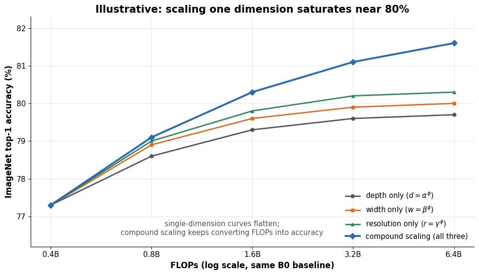
    Line chart of ImageNet top-1 accuracy against FLOPs on a log axis for depth-only, width-only, resolution-only, and compound scaling, with the single-dimension curves flattening near 80 percent while compound scaling keeps rising past 81 percent

    Figure 1: Illustrative accuracy-versus-compute curves from the same B0 baseline: depth-only, width-only, and resolution-only scaling flatten near 80% top-1, while compound scaling keeps converting FLOPs into accuracy.

    The constraint has a direct cost interpretation. A standard convolution’s FLOPs scale linearly with the number of layers and quadratically with both channel count and spatial size, so total compute grows like d \cdot w^{2} \cdot r^{2}. Forcing \alpha \cdot \beta^{2} \cdot \gamma^{2} \approx 2 therefore makes \phi a clean compute dial: each additional unit costs about 2x the FLOPs, and the exponents decide how that doubled budget is split across the three dimensions. The exponents are searched once, on a model cheap enough that a small grid over \alpha, \beta, \gamma is affordable.

    Mathematical Formulation:
    d = \alpha^{\phi}
    w = \beta^{\phi}
    r = \gamma^{\phi}
    \alpha \cdot \beta^{2} \cdot \gamma^{2} \approx 2
    \mathrm{FLOPs}(\phi) \approx 2^{\phi} \cdot \mathrm{FLOPs}(0)

    Where:

    • d, w, and r are the multipliers applied to the baseline’s layer count per stage, channel count per layer, and input side length.
    • \phi is the user-chosen compound coefficient that sets the resource budget; \phi = 0 recovers the baseline B0.
    • \alpha, \beta, \gamma are constants from a small grid search on B0 with \alpha \geq 1, \beta \geq 1, \gamma \geq 1; the published values are 1.2, 1.1, and 1.15.
    • Convolution cost scales as d \cdot w^{2} \cdot r^{2}, so the product constraint is what turns \phi into an approximate doubling of FLOPs per unit.
    Schematic comparing the B0 baseline, drawn as a small input square feeding four short blocks, with the scaled B7 network, drawn as a larger input square feeding six taller blocks

    Figure 2: The same topology at two budgets: a bigger input square (resolution), taller blocks (width), and more blocks (depth) all grow together instead of one dimension racing ahead.

    ModelDepthWidthResolutionFLOPsImageNet Top-1
    B01.0x1.0x2240.39B77.1%
    B31.4x1.2x3001.8B81.6%
    B52.2x1.6x4569.9B83.6%
    B73.1x2.0x60037B84.3%

    Two caveats matter in practice. The released coefficients are rounded rather than exact powers of a single \phi, so treat the formula as the design principle and the published table as the shipped configuration. More importantly, the objective is FLOPs, not latency or memory: depthwise separable convolutions have low arithmetic intensity and underuse GPU and TPU matrix units, and activation memory grows with r^{2}, so the largest variants train slowly and can exhaust device memory. EfficientNetV2 addressed exactly this by replacing early MBConv stages with Fused-MBConv, capping the maximum image size, and adding training-aware search plus progressive resizing.


    Login to view more content
  • DL0072 Inception Module

    What is the Inception module, and how does it use parallel convolutions of different sizes?

    Answer

    The Inception module is the building block of GoogLeNet: instead of committing a layer to one kernel size, it runs several convolutional branches in parallel over the same input (1×1, 3×3, 5×5, plus a 3×3 max-pool path) and concatenates their outputs along the channel axis. Every branch uses stride 1 with padding chosen so all branches emit the same spatial size, which is what makes the concatenation legal. The naive form is prohibitively expensive because the 5×5 branch convolves over the full input depth, so the practical module inserts 1×1 convolutions as channel bottlenecks before the 3×3 and 5×5 convolutions and after the pooling path. The next layer therefore sees features at several receptive-field sizes at once, and the learned weights decide how much of each scale to use rather than the architect fixing one kernel per layer.

    (1) Parallel Multi-Scale Branches: the 1×1, 3×3, 5×5, and pooling paths all read the identical input tensor, so one module covers several receptive fields; a face at 20 px and one at 60 px are both matched inside the same layer.
    (2) Channel-Wise Concatenation: branches keep H and W identical (stride 1, pad 1 for 3×3, pad 2 for 5×5), and outputs are stacked on the channel dimension, so module output depth is the sum of branch depths, not their average.
    (3) 1×1 Bottlenecks: convolution cost is linear in C_{in} C_{out} k^2, so projecting 192 channels down to 16 before the 5×5 conv cuts that branch roughly 10x with a small accuracy cost.
    (4) Dense Ops, Sparse Intent: the design approximates a sparse, locally-optimal connectivity structure using dense operations that BLAS and cuDNN execute efficiently, which is why GoogLeNet reached top ILSVRC-2014 accuracy at about 5M parameters, roughly 12x fewer than AlexNet.

    Two side-by-side block diagrams of an Inception module: on the left the naive version sends the 28x28x192 input straight into 1x1, 3x3, 5x5 convolutions and a 3x3 max pool before filter concatenation; on the right the dimension-reduced version inserts 1x1 convolutions with 96 and 16 channels before the 3x3 and 5x5 convolutions and a 32-channel 1x1 projection after the pool

    Figure 1: Naive versus dimension-reduced Inception module. The 1×1 convolutions shrink channel depth before the expensive kernels and project the pooled path, so concatenation does not grow depth without bound.

    The pooling branch is the reason the naive module is unstable when stacked: max pooling preserves its input depth, so every module would add at least the full input depth back into the concatenated output and channel count would grow monotonically with depth. The 1×1 projection after the pool fixes this, and the same trick applied before the 3×3 and 5×5 convolutions is where nearly all the savings come from. Take the classic Inception (3a) block with a 28 \times 28 \times 192 input and a 5×5 branch producing 32 maps.

    Mathematical Formulation:
    y = \mathrm{concat}(y_1, y_3, y_5, y_p)
    C = H_o W_o C_{out} k^2 C_{in}
    C_{naive} = 28^2 \cdot 32 \cdot 5^2 \cdot 192 \approx 120 \times 10^6
    C_{reduce} = 28^2 \cdot 16 \cdot 1^2 \cdot 192 \approx 2.4 \times 10^6
    C_{conv} = 28^2 \cdot 32 \cdot 5^2 \cdot 16 \approx 10.0 \times 10^6

    Where:

    • y_1, y_3, y_5, y_p are the outputs of the 1×1, 3×3, 5×5, and pooling branches, and \mathrm{concat} stacks them on the channel axis, which requires all four to share the same H_o \times W_o.
    • C counts multiply-adds for one convolution, with H_o W_o the output spatial size, C_{in} and C_{out} the input and output channels, and k the kernel width.
    • C_{naive} is the 5×5 branch applied to all 192 input channels; C_{reduce} is the 1×1 projection to 16 channels and C_{conv} the 5×5 conv on those 16, summing to about 12.4 \times 10^6, roughly a tenth of the naive branch.
    Grouped bar chart of multiply-adds in millions per Inception 3a branch, naive versus dimension-reduced: 1x1 branch 9.6 and 9.6, 3x3 branch 173.4 and 101.2, 5x5 branch 120.4 and 12.4, pool branch 0 and 4.8, module total 303.5 and 128.0

    Figure 2: Multiply-adds per branch for Inception (3a) on a 28 \times 28 \times 192 input. The bottlenecks cut the 5×5 branch from about 120M to 12M and the module total from about 304M to 128M, while also shrinking output depth from 416 to 256 channels.

    Branch1×1 ReductionMain OperationOutput ChannelsMultiply-Adds
    Point-wisenone needed1×1 conv, 64 filters649.6M
    Medium scale192 to 963×3 conv, 128 filters, pad 1128101.2M
    Large scale192 to 165×5 conv, 32 filters, pad 23212.4M
    Pooling192 to 32, after the pool3×3 max pool, stride 1, pad 1324.8M
    Concatenatedchannel-axis concat, 28×28 preserved256128M

    Login to view more content
  • DL0071 VGG vs GoogLeNet vs ResNet

    Compare VGG, GoogLeNet/Inception, and ResNet: what key problem did each architecture address?

    Answer

    The three architectures answer three different questions that the ImageNet era asked in sequence. VGG (2014) asked whether depth alone helps and showed that stacking small 3×3 convolutions to 16 or 19 weight layers beats wide shallow filters, but it paid for that with 138M parameters and 15.3 GFLOPs, roughly 90% of the parameters sitting in three fully connected layers. GoogLeNet/Inception (2014) asked how to get depth and multi-scale receptive fields cheaply: parallel 1×1, 3×3, 5×5, and pooling branches inside one Inception module, with 1×1 bottleneck convolutions cutting channel depth before the expensive kernels, plus global average pooling replacing the fully connected head, giving better accuracy than VGG with about 6.8M parameters and 1.5 GFLOPs. ResNet (2015) asked why depth stopped paying off past roughly 20 to 30 layers and identified the degradation problem: a 56-layer plain net reaches higher training error than a 20-layer one, so this is an optimization failure, not overfitting. Its fix, the identity shortcut y = \mathcal{F}(x) + x, makes each block learn a residual and gives gradients a direct path, which made 152-layer and even 1000-layer networks trainable.

    (1) VGG, Depth Through Uniformity: three stacked 3×3 layers match the 7×7 receptive field with fewer parameters and two extra nonlinearities, proving that a simple repeated motif scales; the cost is a parameter-heavy fully connected head and no answer to what happens beyond ~19 layers.
    (2) Inception, Depth Under a Compute Budget: the module runs several kernel sizes in parallel so the network does not have to choose one scale per layer, and 1×1 reduce → 5×5 conv keeps the cost of the wide branches roughly an order of magnitude lower than the naive version.
    (3) ResNet, Depth Without Degradation: residual blocks reframe the layer’s job as learning a correction to identity, so adding layers can never be worse than copying the input; combined with batch normalization and bottleneck blocks (1×1, 3×3, 1×1), it made very deep training routine.

    Parameter Arithmetic:
    3 \times 3^2 C^2 = 27 C^2
    1 \times 7^2 C^2 = 49 C^2
    5^2 \cdot 192 \cdot 32 = 153{,}600
    192 \cdot 16 + 5^2 \cdot 16 \cdot 32 = 15{,}872

    Where:

    • C is the channel count held constant across the stack, so the first two lines compare three 3×3 layers against one 7×7 layer of identical receptive field: about 45% fewer weights and two extra ReLUs.
    • The third line is the naive Inception 5×5 branch: 192 input channels, 32 output channels, 5^2 spatial taps.
    • The fourth line inserts a 1×1 reduce to 16 channels first, so the same branch costs 15,872 weights, roughly 10\times cheaper; this bottleneck is what let GoogLeNet run 22 layers at 1.5 GFLOPs.
    Scatter plot of ImageNet top-5 error against parameter count on a log scale for VGG-16 at 138M parameters and 7.3 percent, GoogLeNet at 6.8M and 6.7 percent, ResNet-50 at 25.6M and 5.25 percent, and ResNet-152 at 60.2M and 4.49 percent

    Figure 1: Accuracy did not come from parameter count: GoogLeNet beats VGG-16 with about 20\times fewer parameters, and ResNet improves again at moderate size. Evaluation protocols differ slightly across the original papers, so read the trend rather than the decimals.

    The residual idea is the one that generalized furthest. Writing a block as y = \mathcal{F}(x, \{W_i\}) + x means the optimizer only has to push \mathcal{F} toward zero to recover the identity mapping, which is exactly the solution the deeper plain net failed to find. The gradient view is just as important: the identity term contributes an ungated path so the signal reaching early layers cannot vanish through repeated multiplication by small Jacobians. In practice the projection shortcut (1\times1 convolution with stride 2) handles the stage boundaries where spatial size and channel count change.

    Residual Formulation:
    y = \mathcal{F}(x, \{W_i\}) + x
    \frac{\partial L}{\partial x} = \frac{\partial L}{\partial y}\left(I + \frac{\partial \mathcal{F}}{\partial x}\right)

    Where:

    • x is the block input, y its output, and \mathcal{F} the two or three stacked convolutions with weights \{W_i\}.
    • I is the identity Jacobian of the shortcut; it keeps the gradient norm from collapsing even when \partial \mathcal{F} / \partial x is tiny, which is why depth beyond 100 layers becomes trainable.
    • L is the training loss; when shapes differ across a stage, x is replaced by W_s x with a projection shortcut.
    Schematic training error curves over 160 epochs: a 56-layer plain network plateaus at a higher training error than a 20-layer plain network, while a 56-layer ResNet reaches the lowest training error

    Figure 2: Schematic of the degradation problem: the deeper plain network settles at higher training error than the shallower one, ruling out overfitting; the residual version of the same depth trains to the lowest error.

    AspectVGG (2014)GoogLeNet / Inception (2014)ResNet (2015)
    Key problem addressedDoes depth with small kernels beat shallow wide kernels?How to buy depth and multiple scales on a fixed compute budgetDegradation: deeper plain nets train worse
    Signature componentUniform 3×3 conv stacks plus 2×2 max poolInception module with 1×1 bottlenecks, global average poolingIdentity shortcut, bottleneck block (1×1, 3×3, 1×1), batch norm
    Depth16 or 19 weight layers22 layers18 to 152, and 1000+ in experiments
    Parameters / compute138M, 15.3 GFLOPs~6.8M, 1.5 GFLOPs25.6M, 3.8 GFLOPs (ResNet-50)
    Main drawbackHuge FC head, memory hungry, stalls past ~19 layersHand-tuned, irregular module; harder to modify or scaleStill heavy for edge devices; deep variants give diminishing returns
    Lasting legacy3×3 as the default kernel; perceptual loss backbone1×1 channel bottlenecks; no-FC classification headsResidual connections in nearly every modern net, including Transformers

    Login to view more content
  • DL0064 CNNs Object Detection and Segmentation

    What is the role of CNNs in object detection and segmentation?

    Answer

    In object detection and segmentation, a CNN commonly acts as a spatial feature extractor that converts pixels into a hierarchy of increasingly semantic feature maps. Detection heads use those features to classify objects and localize bounding boxes, while segmentation heads upsample and fuse spatial detail to predict per-pixel classes or instance-specific masks. Multiscale features are important because small objects need high-resolution maps and large objects benefit from deeper receptive fields. CNNs are therefore the backbone and often part of the head, but proposal logic, feature pyramids, decoders, and task losses complete the system; modern vision Transformers can also replace or complement the CNN backbone.

    (1) Shared Backbone: Convolutions provide translation-equivariant local processing and reusable feature maps at several strides.
    (2) Detection Role: One-stage or region-based heads turn features into class scores and box coordinates, often using multiscale pyramids.
    (3) Segmentation Role: Dense decoders combine semantic context with fine spatial detail for semantic labels, instance masks, or panoptic outputs.

    CNN multiscale backbone branching into object detection and image segmentation heads.

    Figure 1: A shared convolutional feature hierarchy supports two different outputs: sparse boxes and classes versus dense semantic or instance masks.

    Mathematical Formulation:
    F_l=\mathrm{CNN}_l(I)
    (\hat b,\hat p)=H_{\mathrm{det}}(\{F_l\})
    \hat M=H_{\mathrm{seg}}(\{F_l\})
    \hat M\in\mathbb{R}^{H\times W\times K}

    Where:

    • I is the input image and F_l is the backbone feature map produced by stage l.
    • \{F_l\} is the multiscale feature set supplied to task heads.
    • H_{\mathrm{det}} is the detection head, with \hat b denoting predicted boxes and \hat p predicted class probabilities.
    • H_{\mathrm{seg}} is the segmentation head and \hat M is its dense output mask or logit tensor.
    • H and W are output height and width, while K is the number of semantic classes or mask channels.
    Flowchart comparing CNN processing for detection, semantic segmentation, and instance segmentation.

    Figure 2: Task-specific paths after the backbone show what each head must predict and how its output aligns with the input image.


    Login to view more content
  • DL0061 Channel and Spatial Attention

    Explain channel attention and spatial attention in CNNs. What information does each mechanism model?

    Answer

    Channel attention learns which feature channels are important, answering what semantic responses should be emphasized. It compresses spatial dimensions into channel descriptors, transforms them with a small gating network, and multiplies the resulting weights into the feature tensor. Spatial attention learns where informative regions occur by compressing or projecting the channel dimension and producing an H\times W mask. Modules such as SE use channel attention, while CBAM applies channel attention followed by spatial attention to refine both feature type and location.
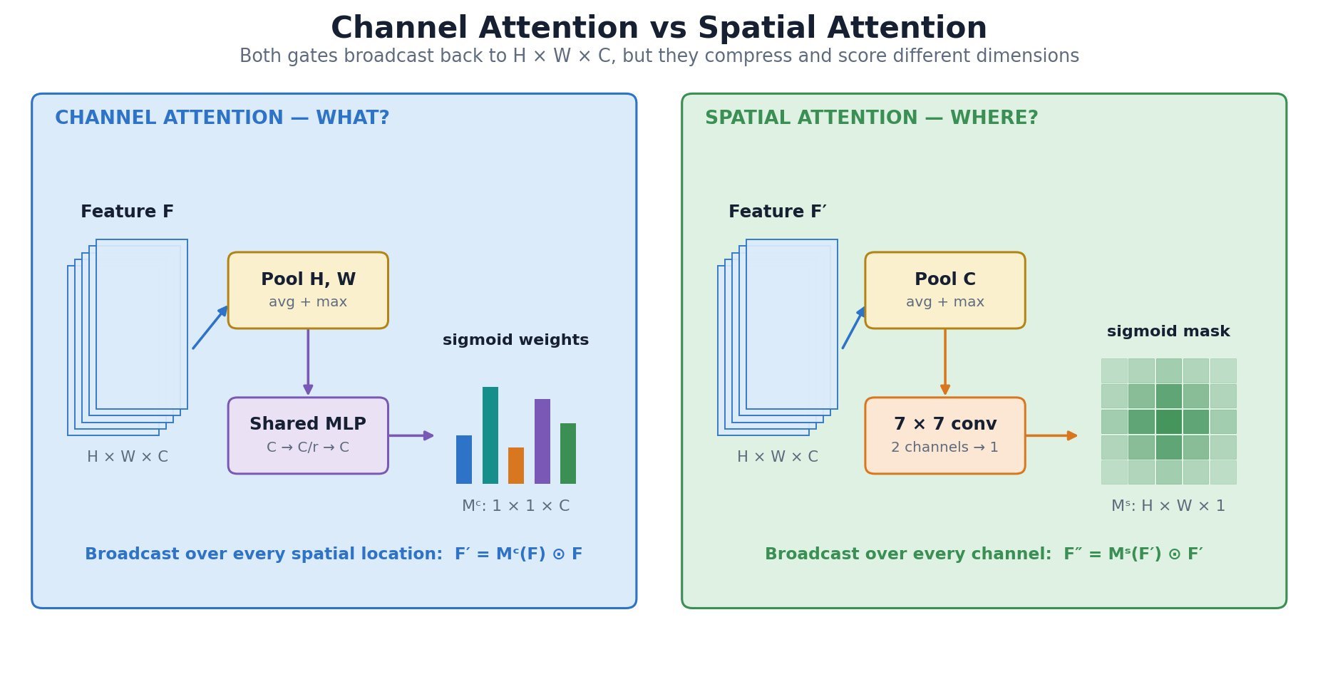
    (1) Channel Gate: Global pooling summarizes each channel; an MLP or 1D convolution captures inter-channel dependence and outputs C multiplicative weights.
    (2) Spatial Gate: Average/max pooling or learned projection across channels produces spatial descriptors that a convolution maps to one H\times W attention mask.
    (3) Residual Placement: Attention usually modulates an existing feature tensor and is often inserted inside a residual block; sigmoid gates reweight rather than replace the underlying features.

    Channel attention and spatial attention mechanisms with tensor reductions and broadcast multiplication.

    Figure 1: Parallel tensor-shape explanation of what channel attention selects and where spatial attention focuses.

    Mathematical Formulation:
    M_c(F)=\sigma\!\left(\mathrm{MLP}(\mathrm{AvgPool}_{hw}(F))+\mathrm{MLP}(\mathrm{MaxPool}_{hw}(F))\right)
    M_s(F)=\sigma\!\left(f^{7\times7}([\mathrm{AvgPool}_{c}(F);\mathrm{MaxPool}_{c}(F)])\right)

    Where:

    • F\in\mathbb{R}^{H\times W\times C} is the input feature map with height H, width W, and C channels.
    • M_c(F)\in\mathbb{R}^{1\times1\times C} is the channel mask; spatial average/max pooling and the shared \mathrm{MLP} produce channel logits.
    • M_s(F)\in\mathbb{R}^{H\times W\times1} is the spatial mask; channel pooling outputs are concatenated by [\,;\,] and filtered by f^{7\times7}.
    • \sigma is the sigmoid function; M_c broadcasts over H,W, while M_s broadcasts over C.
    Sequential CBAM channel-then-spatial attention flowchart.

    Figure 2: CBAM data flow from input feature through channel gating, spatial gating, residual refinement, and output.


    Login to view more content
  • DL0060 Depthwise Separable Convolution

    What is depthwise separable convolution, and where is it commonly used?

    Answer

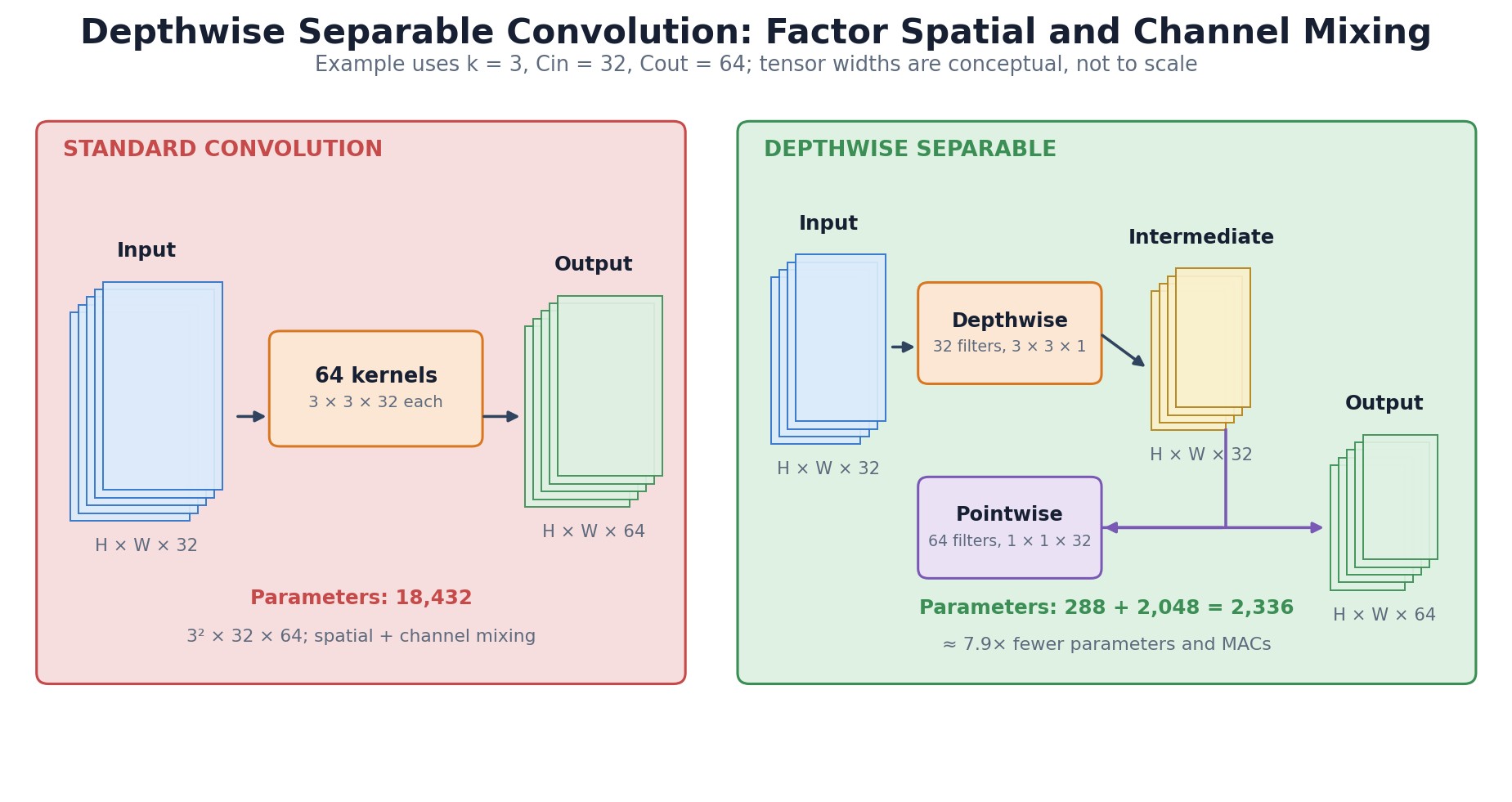
    Depthwise separable convolution factorizes a standard convolution into a depthwise spatial operation and a pointwise channel-mixing operation. The depthwise stage applies one k\times k filter per input channel, so it learns spatial patterns independently; the 1\times1 pointwise stage combines those channel responses into new output channels. This factorization can reduce multiply-accumulates and parameters by almost the kernel area when channel counts are large. It is common in MobileNet, Xception, EfficientNet-style mobile blocks, and edge models where latency, power, and model size matter.

    (1) Depthwise Stage: With depth multiplier one, C_{in} independent k\times k filters produce C_{in} spatially filtered maps and do not mix channels.
    (2) Pointwise Stage: A 1\times1 convolution applies a learned C_{in}\times C_{out} channel transformation independently at every spatial position.
    (3) Real Hardware: Lower arithmetic cost does not guarantee proportional speedup because memory traffic, kernel launch overhead, vectorization, and accelerator support can dominate.

    Standard convolution compared with depthwise and pointwise factorization.

    Figure 1: Tensor-level view of spatial filtering per channel followed by 1×1 channel mixing, with parameters and MACs.

    Mathematical Formulation:
    \mathrm{MACs}_{std}=HWk^2C_{in}C_{out}
    \mathrm{MACs}_{sep}=HW\left(k^2C_{in}+C_{in}C_{out}\right)
    \frac{\mathrm{MACs}_{sep}}{\mathrm{MACs}_{std}}=\frac{1}{C_{out}}+\frac{1}{k^2}

    Where:

    • \mathrm{MACs}_{std} and \mathrm{MACs}_{sep} count multiply-accumulates for standard and depthwise-separable convolution.
    • H and W are output height and width, and k is the square spatial-kernel width.
    • C_{in} and C_{out} are input and output channel counts; the formula assumes depth multiplier 1.
    • For k=3 and large C_{out}, the ratio approaches 1/9.
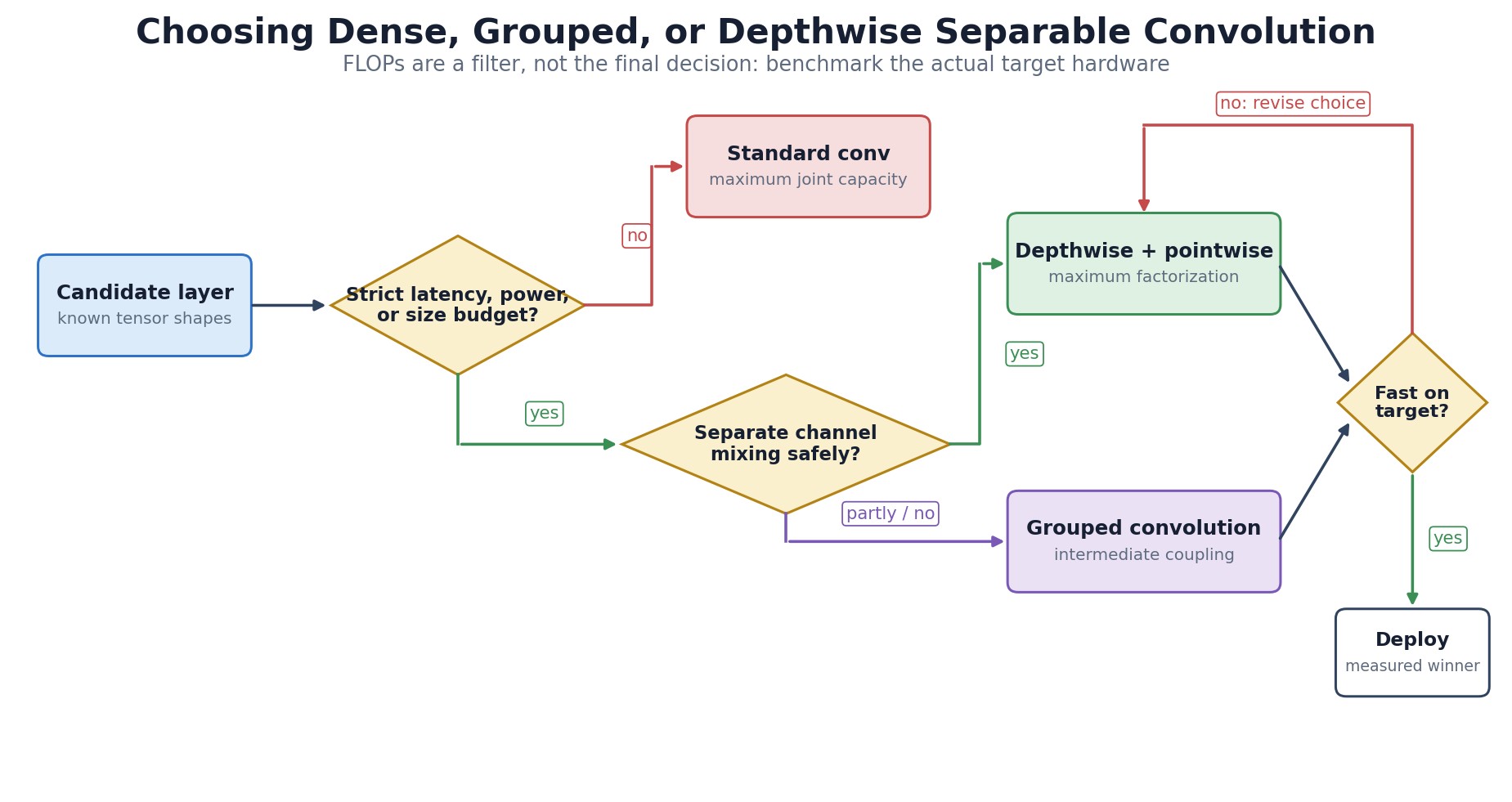
    Decision flowchart for choosing standard, grouped, or depthwise separable convolution.

    Figure 2: Architecture decision based on efficiency target, channel interaction, hardware kernels, and measured latency.


    Login to view more content
  • DL0059 Transposed Convolution

    What is a transposed convolution (sometimes called deconvolution), and when is it used?

    Answer

    A transposed convolution is a learnable linear operator whose matrix is the transpose of the matrix representing a corresponding forward convolution. Operationally, each input value scatters a scaled kernel into an output grid, with stride controlling the spacing and overlapping contributions summed. It can increase spatial resolution, but it is not a mathematical inverse and does not recover information destroyed by downsampling. It is commonly used in semantic-segmentation decoders, generative models, learned reconstruction, and other architectures that map low-resolution features to higher-resolution outputs.

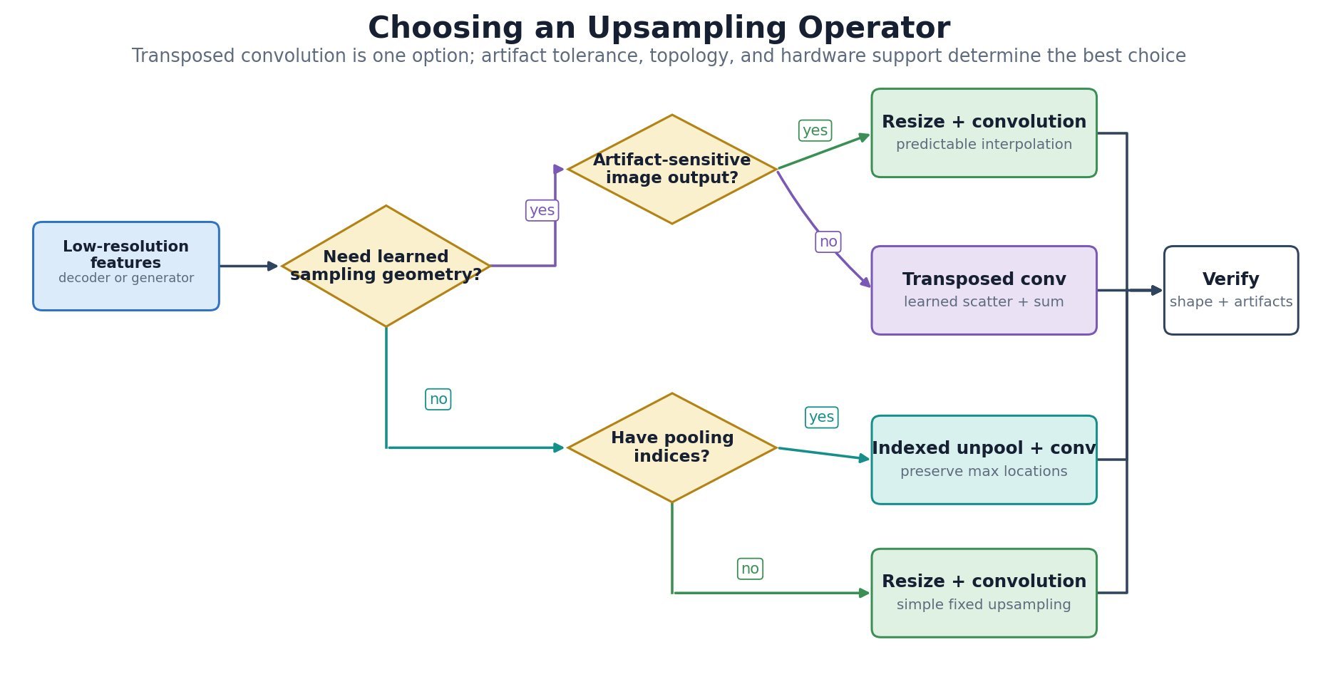
    (1) Learned Upsampling: Unlike fixed nearest-neighbor or bilinear interpolation, the layer learns how feature values contribute to surrounding output positions.
    (2) Output Geometry: Kernel size, stride, padding, dilation, and output padding jointly determine the output shape; output padding resolves shape ambiguity but does not add zero-valued borders.
    (3) Artifact Risk: Uneven overlap occurs when the kernel size is not divisible by stride and can produce checkerboard artifacts, especially in image generators.

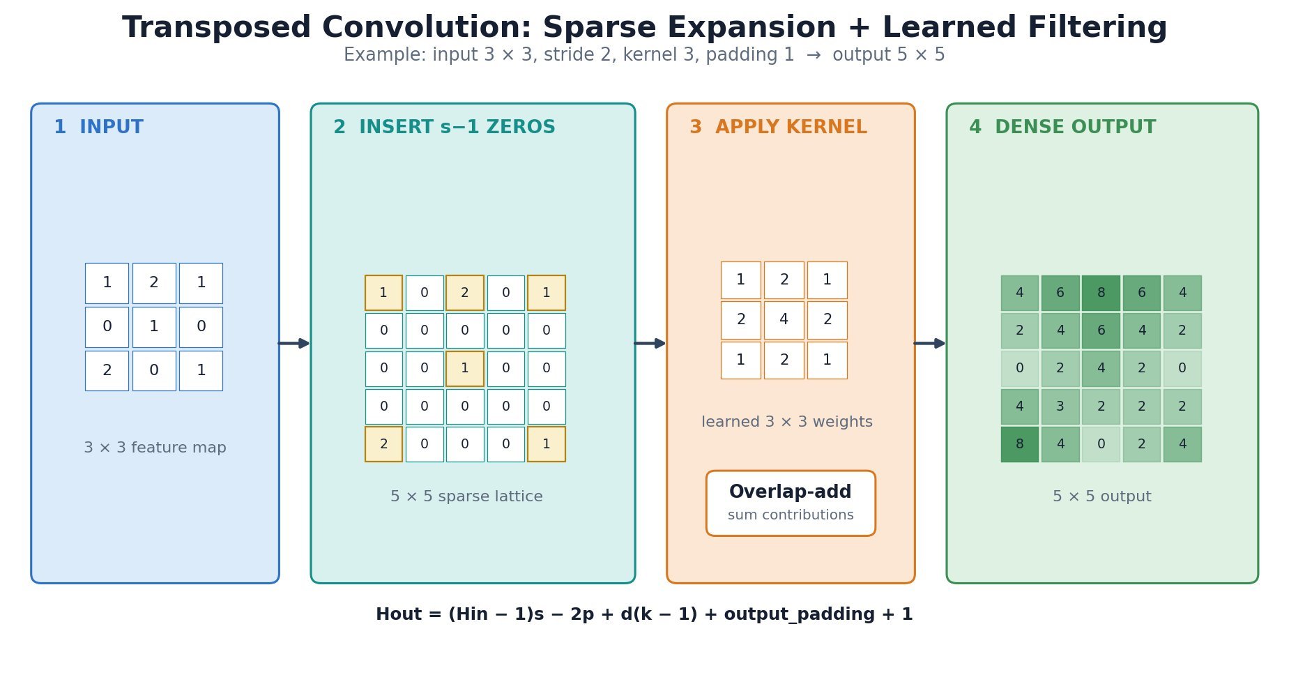
    Transposed convolution shown as zero insertion, kernel application, and overlap summation.

    Figure 1: A stride-2 transposed convolution decomposed into sparse expansion and learned filtering, including output-shape arithmetic.

    Mathematical Formulation:
    H_{out}=(H_{in}-1)s-2p+d(k-1)+p_{out}+1

    Where:

    • H_{in} and H_{out} are the input and output sizes along one spatial axis.
    • s is stride, p is padding, d is dilation, and k is kernel size.
    • p_{out} is output padding used to choose among otherwise ambiguous valid output sizes; it does not append learned pixels.
    • The formula applies independently to width and, for 3D layers, depth by replacing H with the corresponding axis size.
    Upsampling-method decision flowchart comparing transposed convolution, resize-convolution, and unpooling.

    Figure 2: Selection guide based on learned reconstruction, artifact sensitivity, pooling indices, and deployment constraints.


    Login to view more content
  • DL0058 Feature Pyramid Network

    What is a Feature Pyramid Network (FPN) in the context of CNNs, and why is it useful for dense prediction?

    Answer

    A feature pyramid network (FPN) builds a hierarchy of semantically strong feature maps at multiple spatial resolutions. A bottom-up backbone produces progressively smaller maps with richer semantics; a top-down pathway upsamples deep features and merges them with same-resolution lateral projections from earlier stages. The resulting P_2\text{--}P_5 maps combine localization detail with high-level context. Detection, instance segmentation, and keypoint heads can then select a pyramid level appropriate to each object or region scale.

    (1) Bottom-up Hierarchy: Backbone stages C_2\text{--}C_5 reduce spatial resolution while increasing receptive field and semantic abstraction.
    (2) Top-down Fusion: Nearest-neighbor upsampling and 1×1 lateral projections align channel widths before element-wise addition; a 3×3 convolution commonly smooths each merged map.
    (3) Scale Assignment: Small objects use high-resolution levels such as P_2 or P_3, while large objects use coarser levels such as P_4 or P_5.

    Feature Pyramid Network architecture with bottom-up, lateral, and top-down paths.

    Figure 1: FPN construction showing tensor resolution, lateral 1×1 projection, top-down upsampling, fusion, and 3×3 smoothing.

    Mathematical Formulation:
    P_l=\mathrm{Conv}_{3\times3}\!\left(\mathrm{Conv}_{1\times1}(C_l)+\mathrm{Up}_2(P_{l+1})\right)
    k=\left\lfloor k_0+\log_2\!\left(\frac{\sqrt{wh}}{224}\right)\right\rfloor

    Where:

    • C_l is the bottom-up backbone feature and P_l is the fused pyramid output at level l.
    • \mathrm{Conv}_{1\times1} aligns channel width, \mathrm{Up}_2 doubles spatial resolution, and \mathrm{Conv}_{3\times3} smooths the merged feature.
    • k is the assigned pyramid level, k_0 is the reference level, and w,h are the region width and height.
    • 224 is the canonical reference scale and \lfloor\cdot\rfloor maps the continuous log-scale value to a discrete level.
    Feature pyramid scale-selection flowchart for small, medium, and large objects.

    Figure 2: How object size directs prediction heads toward fine, medium, or coarse pyramid levels.


    Login to view more content
  • DL0057 2D VS 3D Convolutions

    What is the difference between 2D and 3D convolutions, and when would you use each?

    Answer

    A 2D convolution slides a kernel across height and width, while aggregating all input channels at each spatial location. A 3D convolution slides across depth or time as well as height and width, so it learns joint spatiotemporal or volumetric features. Use 2D convolution for ordinary images, per-frame video processing, or slice-wise analysis when cross-slice context is unnecessary. Use 3D convolution for videos, CT/MRI volumes, or occupancy grids when local relationships along the third axis carry essential information and the additional memory and compute are affordable.

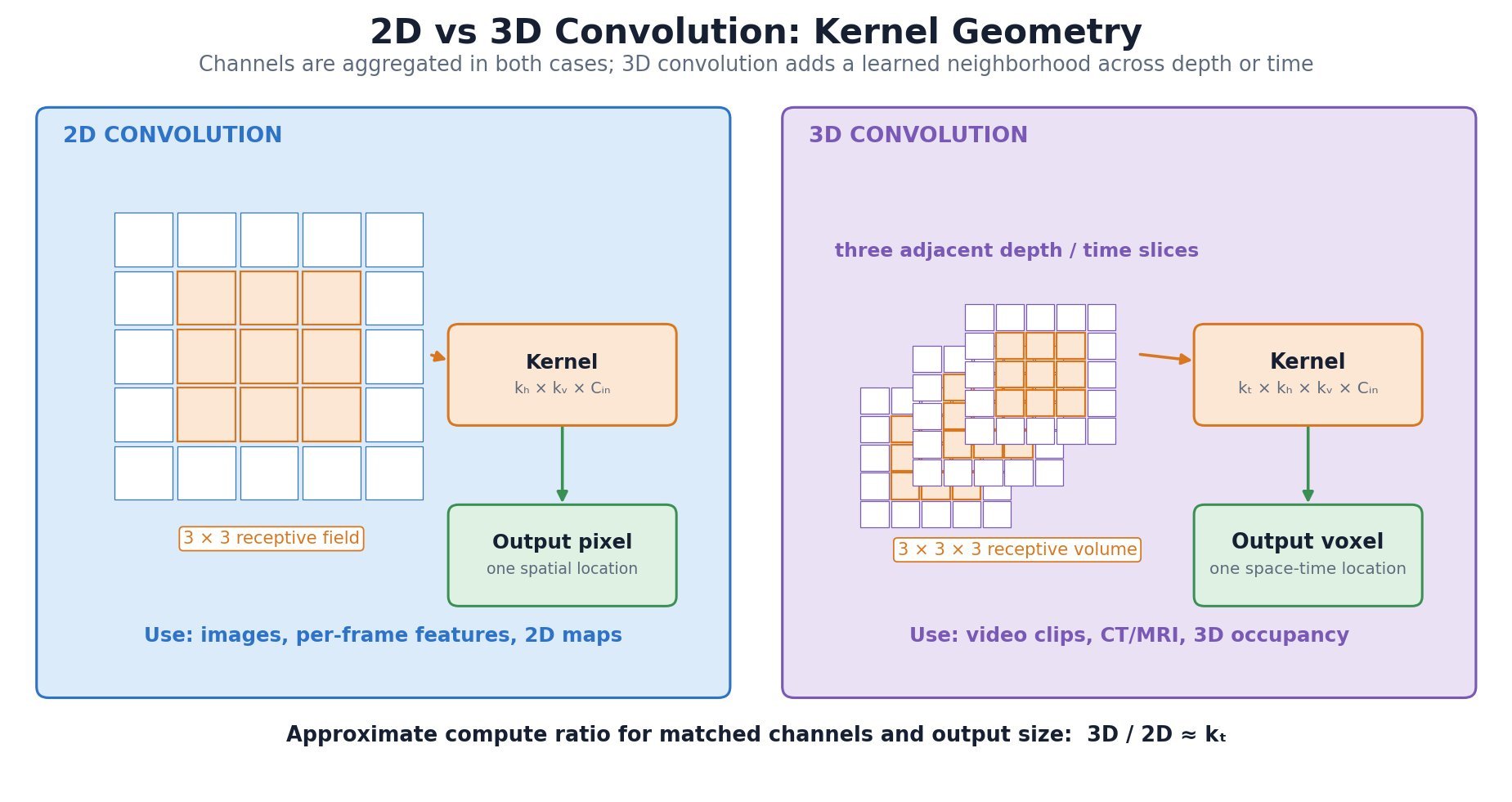
    (1) Kernel Geometry: A 2D kernel has spatial extent k_h\times k_w; a 3D kernel adds k_d and jointly traverses depth or time.
    (2) Data Semantics: The third axis should represent an ordered neighborhood such as adjacent frames or slices, not an unordered feature channel.
    (3) Trade-off: 3D convolution captures motion or volumetric continuity directly but costs roughly k_d times more than a comparable 2D layer and stores larger activation volumes.

    Side-by-side 2D image kernel and 3D spatiotemporal kernel receptive fields.

    Figure 1: Kernel geometry and output formation for 2D spatial convolution and 3D spatiotemporal convolution.

    Mathematical Formulation:
    Y_{o,d,h,w}=\sum_{c=1}^{C_{in}}\sum_{\delta_d,\delta_h,\delta_w}K_{o,c,\delta_d,\delta_h,\delta_w}X_{c,d+\delta_d,h+\delta_h,w+\delta_w}

    Where:

    • X and Y are the input and output tensors, while K is the learned 3D convolution kernel.
    • o indexes output channels and c\in\{1,\ldots,C_{in}\} indexes input channels.
    • d,h,w index output depth/time, height, and width; \delta_d,\delta_h,\delta_w range over the kernel support along those axes.
    • For a 2D convolution, d and \delta_d are removed, leaving only spatial indices h,w; stride, padding, and dilation modify each active index mapping.
    Decision flowchart for selecting 2D, 3D, or factorized convolution.

    Figure 2: Selection guide based on third-axis semantics, required context, resource budget, and deployment constraints.


    Login to view more content
  • DL0024 Fixed-size Input in CNN

    What is the “dilemma of fixed-size input” for CNNs? How is it typically resolved?

    Answer

    The dilemma of fixed-size input is the constraint that classic CNN classifiers (VGG, early ResNets) only accept images of one predetermined resolution: the fully connected head has a weight matrix whose input dimension equals the flattened feature-map size, and that size is only constant if every input image has the same H \times W. Real-world images arrive in arbitrary sizes, so they must be resized or cropped first, distorting aspect ratios, discarding small objects, or cutting content away.

    (1) The FC Head Is the Bottleneck: Convolutions themselves handle any spatial size; only the flatten + FC stage pins the input dimensions.
    (2) Preprocessing Costs Information: Resizing squishes content and can erase small objects; cropping keeps resolution but discards everything outside the window.
    (3) Structural Fixes Exist: Replace or decouple the FC head (GAP, fully convolutional designs, or adaptive pooling) and the network accepts variable sizes natively.

    Three panels showing an original scene with one large and several small objects, a heavily downsampled version where the small objects disappear, and a center crop where objects near the edges are cut away.

    Figure 1: Both standard fixes hurt: downsampling erases small objects; cropping amputates anything near the border.

    Mathematical Formulation (Why the FC Head Fixes the Size):
    z = W \cdot \mathrm{vec}(X) + b, \quad X \in \mathbb{R}^{H \times W \times C}
    \mathrm{GAP}(X)_c = \frac{1}{HW} \sum_{h=1}^{H} \sum_{w=1}^{W} X_{hwc}

    Where:

    • X is the final feature volume; \mathrm{vec}(X) flattens it to HWC values, so W exists only for one specific H \times W.
    • \mathrm{GAP}(X)_c averages channel c over all spatial positions, yielding a C-dimensional vector for any input size.

    Common Solutions: (1) Global Average Pooling: replace the flatten with a per-channel average, so the classifier sees exactly C values regardless of resolution; (2) Fully Convolutional Networks: remove FC layers entirely and let the output scale with the input (standard for segmentation); (3) Adaptive Pooling: pool to a fixed k \times k grid no matter the input size (e.g., nn.AdaptiveAvgPool2d in PyTorch).

    Diagram of a variable-size input feeding three solution paths, global average pooling, fully convolutional network, and adaptive pooling, all converging to a fixed classifier head that accepts any input size.

    Figure 2: Three structural escapes (GAP, FCN, and adaptive pooling) all remove the fixed-size constraint at its source: the FC head.


    Login to view more content