
What is the score-based / score-matching interpretation of diffusion models, as used in systems like Stable Diffusion?
Answer
The score-based view says a diffusion model never learns a density; it learns the score, the gradient of the log density  . This is attractive because the gradient annihilates the intractable normalizing constant: if
  then
then  with no
  anywhere, so an unnormalized energy model becomes trainable. Direct score matching still needs the intractable
  , and the fix is denoising score matching: perturb the data with a known Gaussian kernel, and the score of the perturbed conditional is available in closed form, which reduces the loss to predicting the noise that was added. Because a single small noise level leaves the score undefined off the data manifold and unreliable in low-density regions, the model is trained over a continuum of noise levels, which turns into the forward SDE of Song et al. and makes sampling the simulation of a reverse-time SDE or its deterministic probability-flow ODE. The punchline is that DDPM’s noise-prediction network is the same object in different clothing:
  , so the discrete-time denoising story and the continuous-time score story are two parameterizations of one model.
(1) Model The Gradient, Not The Density: learning  removes the partition function, so the network output is an unconstrained vector field of the same shape as the data.
(2) Denoising Score Matching Makes It Tractable: Vincent’s identity shows that regressing onto  has the same minimizer as matching the true marginal score, and that target is just the scaled added noise.
(3) Multiple Noise Scales Are Essential: real data lies near a low-dimensional manifold where the score is ill-defined, and large noise levels smooth the density so the vector field is informative everywhere and connects separated modes.
(4) Sampling Is Numerical Integration: annealed Langevin dynamics, the reverse SDE, and the probability-flow ODE all consume only the learned score; the ODE additionally gives exact likelihoods and deterministic, invertible latents.
(5) Unifies VE And VP Diffusions: NCSN’s variance-exploding noise ladder and DDPM’s variance-preserving chain are two discretizations of the same SDE family, differing in  ,
,  , and the loss weighting
  .
.
The geometric picture is worth holding onto. The score at a point is the direction of steepest increase in log density, so the learned field points from wherever you are toward nearby high-probability regions, and its magnitude grows as you move into the tails. Sampling then means dropping a Gaussian sample somewhere in space and following that field while injecting just enough noise to keep the chain from collapsing onto a single mode. The reason this needs annealing is that a score trained only at tiny noise is accurate on the data manifold and near-arbitrary far from it, where every initial sample actually starts.
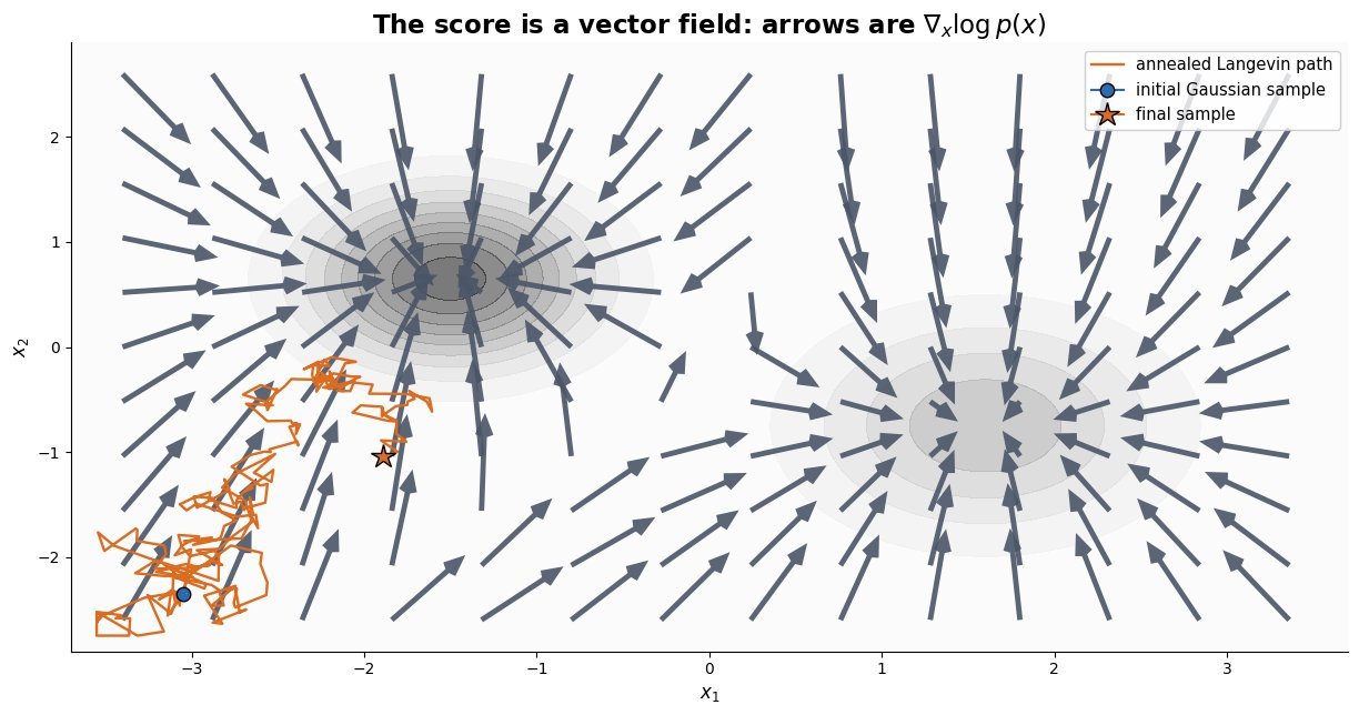
Figure 1: The learned score is a vector field pointing toward high-density regions; a Langevin chain follows it from a random start and ends up distributed according to  , never evaluating the density itself.
Mathematical Formulation:


![\mathcal{L}(\theta) = \mathbb{E}\left[ \lambda_t \left\| s_\theta(x_t,t) + \frac{\epsilon}{\sigma_t} \right\|^2 \right]](https://s0.wp.com/latex.php?latex=%5Cmathcal%7BL%7D%28%5Ctheta%29+%3D+%5Cmathbb%7BE%7D%5Cleft%5B+%5Clambda_t+%5Cleft%5C%7C+s_%5Ctheta%28x_t%2Ct%29+%2B+%5Cfrac%7B%5Cepsilon%7D%7B%5Csigma_t%7D+%5Cright%5C%7C%5E2+%5Cright%5D&bg=ffffff&fg=000&s=3&c=20201002)

![dx = \left[ f - g^2 s_\theta \right] dt + g\,d\bar{w}](https://s0.wp.com/latex.php?latex=dx+%3D+%5Cleft%5B+f+-+g%5E2+s_%5Ctheta+%5Cright%5D+dt+%2B+g%5C%2Cd%5Cbar%7Bw%7D&bg=ffffff&fg=000&s=3&c=20201002)
![dx = \left[ f - \tfrac{1}{2} g^2 s_\theta \right] dt](https://s0.wp.com/latex.php?latex=dx+%3D+%5Cleft%5B+f+-+%5Ctfrac%7B1%7D%7B2%7D+g%5E2+s_%5Ctheta+%5Cright%5D+dt&bg=ffffff&fg=000&s=3&c=20201002)

Where:
 is the network output, a vector with the same shape as
  , approximating the score of the perturbed marginal
  .
. is a clean data point,
  its noisy version, and
  the Gaussian draw.
 and define the noise schedule; variance-preserving keeps
  , variance-exploding fixes
  and grows .
![t \in [0,T]](data:image/svg+xml;base64,PHN2ZyB4bWxucz0iaHR0cDovL3d3dy53My5vcmcvMjAwMC9zdmciIHdpZHRoPSI2MSIgaGVpZ2h0PSIxNyIgdmlld0JveD0iMCAwIDYxIDE3Ij48cmVjdCB3aWR0aD0iMTAwJSIgaGVpZ2h0PSIxMDAlIiBzdHlsZT0iZmlsbDojY2ZkNGRiO2ZpbGwtb3BhY2l0eTogMC4xOyIvPjwvc3ZnPg==) indexes the noise level, with
indexes the noise level, with  essentially pure Gaussian noise;
  is the loss weighting, and the choice
  turns the objective into the plain noise-prediction MSE.
 is the drift and
  the diffusion coefficient of the forward SDE;
  is a Wiener process and
  its reverse-time counterpart, so the second SDE is integrated from
  down to
  .
.- The final line is the reparameterization identity linking the score view to DDPM’s ; required initial condition for sampling:
 for the VE case.
 is the network output, a vector with the same shape as
  , approximating the score of the perturbed marginal
  .
. is a clean data point,
  its noisy version, and
  the Gaussian draw.
 and
and  define the noise schedule; variance-preserving keeps
  , variance-exploding fixes
  and grows
 ![t \in [0,T]](https://s0.wp.com/latex.php?latex=t+%5Cin+%5B0%2CT%5D&bg=ffffff&fg=000&s=2&c=20201002) indexes the noise level, with
indexes the noise level, with  essentially pure Gaussian noise;
  turns the objective into the plain noise-prediction MSE.
 is the drift and
  the diffusion coefficient of the forward SDE;
  is a Wiener process and
  its reverse-time counterpart, so the second SDE is integrated from
  down to
  .
. ; required initial condition for sampling:
  for the VE case.
Figure 2: Why a ladder of noise levels is required: at  the score carries no usable signal away from the data, while at
  the smoothed field points inward from everywhere and bridges the two modes.
| Property | Score SDE (VE, NCSN) | DDPM (VP, noise-pred) | Flow matching |
|---|---|---|---|
| Network output | Score, magnitude scales like 1/sigma_t | Unit-variance noise estimate | Velocity field of a probability path |
| Corruption | Add noise, variance grows to data scale | Shrink signal, keep total variance at 1 | Straight interpolation between data and noise |
| Loss | Weighted denoising score matching | Same loss with weighting sigma_t squared | Regression onto the conditional velocity |
| Sampler | Annealed Langevin or predictor-corrector | Ancestral chain, or DDIM as an ODE | ODE solver on a near-straight path |
| Exact likelihood | Yes, via the probability-flow ODE | Only an ELBO in discrete time | Yes, continuous normalizing flow change of variables |
Leave a Reply