Tag: NN

  • DL0012 Zero Padding

    Why is zero padding used in deep learning?

    Answer

    Zero padding adds rows and columns of zeros around the input before a convolution. In CNNs it preserves spatial dimensions, prevents border information from being under-sampled, allows larger kernels and deeper stacks, and gives explicit control over output size. Beyond CNNs, padding standardizes variable-length sequences so NLP and time-series models can process them in batches.

    (1) Preserves Spatial Dimensions: Without padding (“valid” convolution), a k \times k kernel shrinks the feature map by k - 1 in total per dimension ((k-1)/2 per side) each layer; padding with p = (k-1)/2 keeps the size unchanged.
    (2) Retains Boundary Information: Padded borders let the kernel center on edge pixels, so corners and boundaries are processed as thoroughly as the interior.
    (3) Controls Output Size: Padding decouples output dimensions from kernel size, enabling deeper networks and predictable feature-map shapes.

    Mathematical Formulation:
    n_{out} = \left\lfloor \frac{n_{in} + 2p - k}{s} \right\rfloor + 1

    Where:

    • n_{out} and n_{in} are the output and input spatial sizes.
    • p is the padding width added to each side, k is the kernel size, and s is the stride.
    • “Same” padding for stride 1 uses p = (k-1)/2, giving n_{out} = n_{in}.
    2D convolution example showing a 4x4 input padded with one ring of zeros into 6x6, so a 3x3 kernel produces a same-size 4x4 output.

    Figure 1: Padding a 4 \times 4 input to 6 \times 6 lets a 3 \times 3 kernel output the same 4 \times 4 size instead of shrinking to 2 \times 2.

    Beyond CNNs: In NLP and time-series tasks, zero padding extends shorter sequences to a uniform length for efficient batching. Because padded positions carry no information, models combine padding with attention masks so Transformer self-attention ignores those positions entirely.

    Three panels comparing valid convolution without padding, same convolution with padding, and NLP sequence padding with an attention mask.

    Figure 2: Valid shrinks the map, same preserves it, and sequence padding plus a mask enables batched NLP inputs.


    Login to view more content
  • ML0034 Backpropagation

    What is backpropagation?

    Answer

    Backpropagation (backward propagation of errors) is the algorithm by which neural networks learn: it efficiently computes how much every weight and bias contributed to the prediction error, so an optimizer can adjust each parameter in the direction that reduces the loss. At its core it is the chain rule of calculus applied systematically: after a forward pass computes the output and the loss, a backward pass starts at the output layer, computes the error signal \delta = \partial L / \partial z there, and recursively propagates it backward: each layer’s error is a weighted sum of the next layer’s errors times the local activation derivative, and each weight’s gradient is simply its neuron’s error signal times the input it received. This reuses intermediate results so the cost of computing all gradients is roughly one extra forward pass, which is what makes training deep networks tractable. Gradients then feed an optimizer (SGD, Adam) that performs the actual update w \leftarrow w - \eta \, \partial L / \partial w.

    (1) Forward Pass: Inputs flow through the network producing a prediction; all intermediate activations are cached.
    (2) Backward Pass: The loss error propagates backward via the chain rule: each layer’s \delta is built from the next layer’s.
    (3) Gradient & Update: \partial L / \partial w_i = \delta \cdot x_i; the optimizer subtracts a learning-rate-scaled step.

    Three layer network with forward activations flowing left to right and gradient deltas flowing right to left

    Figure 1: The two passes: activations flow forward (blue) through each layer to the loss; error signals \delta flow backward (orange) along the same edges, and every weight’s gradient combines the forward activation with the backward error.

    Mathematical Formulation:
    z = \sum_{i} w_i x_i + b
    a = f(z)
    \delta = \frac{\partial L}{\partial z} = \frac{\partial L}{\partial a}\, f'(z)
    \delta_j = \Big( \sum_{k} \delta_k \, w_{kj} \Big) f'(z_j)
    \frac{\partial L}{\partial w_i} = \delta \cdot x_i
    \frac{\partial L}{\partial b} = \delta

    Where:

    • z is the pre-activation and a = f(z) the activation of a neuron; L the loss.
    • \delta is the error signal: how much the loss changes per unit change of z; at hidden neuron j it sums contributions \delta_k w_{kj} from all downstream neurons k.
    • x_i is the input feeding weight w_i: the gradient is proportional to it; the bias gradient equals \delta itself.
    Single neuron computation graph with numeric forward values and backward gradients

    Figure 2: One numeric step through a neuron: forward values (blue) compute z = wx + b and a = \sigma(z); backward gradients (orange) multiply local derivatives down the chain: \partial L/\partial w = 0.16 \times 0.5 = 0.08, so the weight updates as w \leftarrow w - \eta \cdot 0.08.


    Login to view more content
  • ML0033 All Zeros Init

    How does initializing all weights and biases to zero affect a neural network’s training?

    Answer

    Initializing every weight and bias to zero creates a fatal symmetry problem: all neurons in a layer compute the same output, receive the same gradient, and update identically, so they remain identical forever. The layer effectively behaves as a single neuron no matter how wide it is, the network cannot learn diverse features, and its representational capacity collapses. The pathology goes further: with zero weights, activations propagate as zero through the layers (for ReLU the forward signal is exactly 0), and gradients backpropagating through zero weights vanish entirely, so training can stall from the very first step. Proper initialization is therefore not a cosmetic choice: random schemes like Xavier/He break the symmetry and set the activation scale so signals flow through the full depth of the network.

    (1) Symmetry: Identical weights → identical outputs → identical gradients → identical neurons forever; width is wasted.
    (2) No Learning Signal: Zero weights kill forward activations and backward gradients (especially with ReLU), stalling training.
    (3) Fix: Small random initialization (Xavier/He) breaks symmetry and keeps activation/gradient variance stable across layers.

    Training and validation accuracy for zero initialization stuck at chance level versus random initialization learning successfully

    Figure 1: Zero versus random initialization on a binary task: with all-zero weights, train and validation accuracy stay pinned at the 0.5 chance level: the network learns nothing; random initialization breaks symmetry and both curves climb above 0.9.

    Mathematical Formulation:
    z_j = \sum_{i} w_{ji} x_i + b_j = 0 \quad \forall j \;\; (\text{all-zero init})
    \frac{\partial L}{\partial w_{ji}} = \delta_j \, x_i
    \delta_j = f'(z_j) \sum_k \delta_k w_{kj} = 0

    Where:

    • w_{ji} is the weight from input i to neuron j, b_j its bias, z_j its pre-activation.
    • \delta_j is the backpropagated error signal of neuron j; with downstream weights w_{kj} = 0 it collapses to 0, so every weight gradient is 0.
    • Even where a gradient exists (first layer before the collapse), every neuron in a layer gets the same gradient and stays identical: the symmetry itself is the deeper failure.

    Login to view more content
  • DL0011 Fully Connected Layer

    Can you explain what a fully connected layer is?

    Answer

    A fully connected (FC) layer, also called a dense layer, is a layer in which every neuron connects to all neurons of the previous layer. It computes a weighted sum of its inputs, adds a bias, and applies an activation function, letting the network learn global combinations of features. FC layers typically appear at the end of a network, mapping extracted features to class scores.

    (1) Dense Connectivity: With n_{in} inputs and n_{out} neurons, the layer holds n_{in} \times n_{out} weights plus n_{out} biases.
    (2) Parameter Heavy: FC layers often dominate model size (e.g., flattening a 7 \times 7 \times 512 map into 1000 classes needs ~25M parameters), which raises overfitting risk.
    (3) Loses Spatial Structure: Inputs must be flattened, discarding spatial layout; Global Average Pooling (GAP) is a parameter-free alternative.

    Mathematical Formulation:
    y = \sigma(Wx + b)
    \#\text{params} = (n_{in} + 1) \times n_{out}

    Where:

    • x \in \mathbb{R}^{n_{in}} is the flattened input vector and y \in \mathbb{R}^{n_{out}} is the output vector.
    • W \in \mathbb{R}^{n_{out} \times n_{in}} is the weight matrix and b \in \mathbb{R}^{n_{out}} is the bias vector.
    • \sigma is a non-linear activation such as ReLU (or softmax at the classifier output).
    Fully connected layer diagram showing every input neuron connected to every output neuron, with the weighted sum and activation annotation.

    Figure 1: In an FC layer, every input neuron connects to every output neuron; each output is \sigma(\sum_j w_j x_j + b).

    Flatten + FC vs GAP + FC: For a CNN head with 7 \times 7 \times 8 feature maps and 6 classes, flattening feeds 392 values to the FC layer, while GAP feeds only 8, a 44× parameter reduction with less overfitting:

    ApproachFC Input SizeFC ParametersSpatial Info
    Flatten + FC7 \times 7 \times 8 = 392(392 + 1) \times 6 = 2358Discarded by flattening
    GAP + FC8 (one per channel)(8 + 1) \times 6 = 54Summarized per channel
    Two CNN head pipelines compared: flatten plus fully connected layer versus global average pooling plus fully connected layer, with parameter counts annotated.

    Figure 2: GAP collapses each feature map to one value before the FC layer, cutting parameters from 2358 to 54 in this example.


    Login to view more content
  • DL0010 Receptive Field

    What is the receptive field in convolutional neural networks, and how do you calculate it?

    Answer

    The receptive field (RF) of a neuron is the region of the input image that can influence that neuron’s activation. It grows with network depth, so deeper layers see larger context and learn more hierarchical features. The RF is computed layer by layer: each layer expands the field according to its kernel size, scaled by the cumulative stride of all preceding layers.

    (1) Definition: The RF is the input region that affects one activation in a given layer; a neuron with a large RF integrates global context.
    (2) Growth Rule: Each layer adds (k_l - 1) \times \prod s_i to the RF, where k_l is the kernel size and the product runs over all previous strides.
    (3) Design Implication: Stacked small kernels grow the RF parameter-efficiently; strided and dilated convolutions grow it much faster.

    Mathematical Formulation:
    RF_l = RF_{l-1} + (k_l - 1) \times \prod_{i=1}^{l-1} s_i

    Where:

    • RF_l is the receptive field size after layer l, with RF_0 = 1 at the input layer.
    • k_l is the kernel size of layer l.
    • s_i is the stride of layer i, and the product accumulates all strides before layer l.
    Stacked feature map rows showing the receptive field of one neuron growing from 3 to 5 to 7 input cells across three 3x3 convolution layers with stride 1.

    Figure 1: With k=3, s=1 per layer, one neuron’s RF grows from 3 to 5 to 7 input cells as layers stack.

    Stride and Dilation Effects: A layer with stride 2 doubles the jump between adjacent neurons, so every subsequent layer adds twice as much to the RF. Dilated convolutions enlarge the kernel’s span by inserting gaps, growing the RF without reducing resolution, which is useful in segmentation.

    Worked receptive field calculation across four layers showing RF values 1, 3, 5, 7, 11 with the contribution of a stride-2 layer multiplying later increments.

    Figure 2: Worked example: a stride-2 layer at l=3 doubles the increment contributed by every later layer, jumping the RF from 7 to 11.

    Real CNN Stacks: In practice, convolutions, pooling, and dilation mix freely: pooling multiplies the jump between neurons, and dilated kernels widen the span, so the RF can reach 22 within just five layers.

    Line chart of receptive field size growing from 1 to 22 across a CNN stack with convolutions, max pooling, and a dilated convolution.

    Figure 3: In a realistic stack, max pooling doubles the jump and dilation (D=2) widens the kernel, pushing the RF from 1 to 22 in five layers.


    Login to view more content
  • DL0004 Small Kernels

    What are the key advantages of using small convolutional kernels, such as 3×3, over utilizing a few larger kernels in deep learning architectures?

    Answer

    Using small convolutional kernels instead of a few larger kernels lets a network reach the same receptive field with fewer parameters, more depth, and more non-linearity. A stack of 3\times3 convolutions matches the spatial coverage of a single large kernel while inserting an activation between each layer, which increases the network’s representational power. This design is the foundation of architectures such as VGG.

    (1) Deeper Networks & More Non-Linearity: Stacking multiple 3\times3 layers (e.g., three of them) creates a deeper network with more non-linear activation functions than a single large kernel.
    (2) Reduced Parameters: Multiple small kernels achieve the same receptive field as a larger one with fewer parameters: two stacked 3\times3 layers use 18\cdot C_{in}\cdot C_{out} weights versus 25\cdot C_{in}\cdot C_{out} for one 5\times5 layer.
    (3) Computational Efficiency: Fewer parameters generally mean lower FLOPs during training and inference.
    (4) Gradual Receptive Field Expansion: Successive 3\times3 convolutions progressively build a larger receptive field while preserving local detail capture, ideal for textures and edges.

    Two stacked 3x3 convolutions viewing the same 5x5 input region as a single 5x5 convolution.

    Figure 1: Two stacked 3\times3 convolutions see the same 5\times5 input region as one 5\times5 convolution, but with an extra non-linearity in between.

    Kernel Composition: Two stacked 3\times3 kernels compose into a single equivalent 5\times5 kernel (their full discrete convolution), which is exactly why the receptive fields match.

    Two all-ones 3x3 kernels composing into an equivalent 5x5 kernel with coefficients formed by their full discrete convolution.

    Figure 2: Two 3\times3 kernels compose into one equivalent 5\times5 kernel; stacking keeps them separate: 18 weights plus an extra non-linearity instead of a 25-weight merge.

    Mathematical Formulation:
    P_k = k^2 \cdot C_{in} \cdot C_{out}
    RF_l = 1 + l\cdot(k-1)
    2 \times 3^2 = 18 \text{ vs } 5^2 = 25
    3 \times 3^2 = 27 \text{ vs } 7^2 = 49

    Where:

    • P_k is the parameter count of one k\times k convolution (ignoring biases).
    • C_{in} and C_{out} are the input and output channel counts.
    • RF_l is the receptive field after l stacked layers; two 3\times3 layers give RF=5, three give RF=7.
    Bar chart comparing parameter counts of 5x5 and 7x7 convolutions against stacked 3x3 convolutions with equal receptive fields.

    Figure 3: For an equal receptive field, stacked 3\times3 convolutions cut parameters by 28% (vs 5\times5) and 45% (vs 7\times7).


    Login to view more content
  • DL0003 1×1 Convolution

    What are the benefits of using 1×1 convolutional layers in deep learning architectures?

    Answer

    A 1×1 convolution (pointwise convolution) operates on the channel dimension at each spatial location, enabling dimensionality control, cross-channel feature fusion, and non-linear mixing, all with minimal computational cost. In architectures like ResNet’s bottleneck block, a 1×1 conv first reduces channels (e.g., 256→64), a 3×3 conv processes the reduced representation, and another 1×1 conv expands back (64→256), restoring capacity while keeping compute manageable. This design allows deeper networks without prohibitive parameter growth.

    (1) Dimensionality Control: 1×1 convolutions can reduce or expand the number of feature maps, trading off representational capacity and computational cost as needed.
    (2) Depth With Controlled Cost: By reducing channel dimensionality before expensive spatial convolutions, 1×1 convs enable deeper architectures without the quadratic growth in channel count that a plain 3 \times 3 block incurs.
    (3) Cross-Channel Feature Fusion: Each output pixel is a learned linear combination of all input channels at that location, enabling rich channel-wise interactions.
    (4) Non-Linear Mixing: When followed by activations (ReLU, etc.), 1×1 convs introduce non-linear channel mixing that enhances model expressiveness.

    1x1 convolution operation showing per-pixel cross-channel weighted sum across input channels to produce one output channel.

    Figure 1: A 1×1 convolution performs a per-pixel weighted sum across all input channels: each output channel is a learned linear combination of every input channel at the same spatial position, preserving H\times W.

    Mathematical Formulation:
    y_{i,j,c_{out}} = \sum_{c_{in}=1}^{C_{in}} w_{c_{in},c_{out}} \cdot x_{i,j,c_{in}} + b_{c_{out}}
    \text{FLOPs}_{1\times1} = H \times W \times C_{in} \times C_{out}

    Where:

    • x_{i,j,c_{in}} is the input activation at spatial position (i,j) in channel c_{in}; y_{i,j,c_{out}} is the output.
    • w_{c_{in},c_{out}} is the 1×1 kernel weight connecting input channel c_{in} to output channel c_{out}; there is no spatial kernel dimension.
    • C_{in} and C_{out} are the input and output channel counts; b_{c_{out}} is the bias for each output channel.
    • H and W are the spatial height and width of the feature map; the operation is equivalent to a fully-connected layer applied per-pixel across channels.
    ResNet bottleneck block showing 1x1 convolutions reducing then expanding channels around a 3x3 convolution.

    Figure 2: ResNet bottleneck block: a 1×1 conv reduces channels (256→64), a 3×3 conv processes the compressed representation, and another 1×1 conv expands back (64→256), with a residual skip connection.


    Login to view more content
  • DL0002 All Ones Init

    What are the potential consequences of initializing all weights to one in a deep learning model?

    Answer

    Initializing all weights to one (or any constant non-zero value) creates a symmetry problem: every neuron in the same layer receives identical gradients, so they learn the same features and cannot develop diverse representations. This limits the network to a single effective feature per layer, severely reducing its representational capacity. Training becomes slow or fails to converge because the optimizer cannot differentiate between neurons. Additionally, constant positive weights can push activations into saturated regions of sigmoid or tanh, worsening vanishing gradients.

    (1) Symmetry Problem: All neurons in a layer receive the same input and the same gradient, so they evolve identically throughout training.
    (2) Limited Representational Capacity: The network behaves as if each layer has only one neuron, making it impossible to capture complex, varied patterns in the data.
    (3) Slow or Failed Convergence: Because neurons cannot differentiate, the loss landscape lacks the diversity needed for gradient descent to find useful minima.
    (4) Activation Saturation: Uniform positive weights shift pre-activation values into the flat tails of sigmoid and tanh, producing vanishing gradients that stall learning.

    Symmetry problem visualization comparing all-ones initialization where neurons collapse versus random initialization with diverse features.

    Figure 1: The symmetry problem: with all-ones weights every neuron computes the same function and receives the same gradient, while random initialization lets each neuron learn a distinct feature.

    Mathematical Formulation:
    \frac{\partial \mathcal{L}}{\partial w_{ij}^{(l)}} = \delta_i^{(l)} \cdot a_j^{(l-1)}
    w_{ij}^{(l)} = 1 \quad \forall\, i,j \implies \delta_i^{(l)} = \delta_j^{(l)} \quad \forall\, i,j

    Where:

    • w_{ij}^{(l)} is the weight from neuron j in layer l-1 to neuron i in layer l.
    • \delta_i^{(l)} is the error signal (delta) for neuron i in layer l.
    • a_j^{(l-1)} is the activation of neuron j in the previous layer.
    • \mathcal{L} is the loss function; when all weights are equal, all delta signals are identical, so every weight updates by the same amount.
    Training loss comparison between ones initialization and random initialization showing slow convergence for constant weights.

    Figure 2: Training loss comparison: ones initialization converges slowly and plateaus at a high loss, while random initialization descends rapidly to a low minimum.


    Login to view more content
  • DL0001 Residual Connection

    Why are residual connections important in deep neural networks?

    Answer

    A residual connection (skip connection) adds a block input to a learned residual transformation, so the block learns an update rather than an entirely new mapping. For a shape-preserving block, the local Jacobian becomes I+J_F, which supplies a direct identity component and creates shorter paths through the computational graph. This usually improves gradient propagation and optimization, but it does not guarantee nonzero or constant gradients: products of residual-block Jacobians can still shrink, grow, or cancel. Residual connections also address the degradation problem, in which adding layers to a plain network can increase training error because the deeper model is difficult to optimize even though an identity extension exists. These properties enabled effective training of ResNet architectures with hundreds of layers.

    (1) Shorter Gradient Paths: An identity shortcut changes the local block Jacobian from J_F to I+J_F. The identity component gives backpropagation additional routes, although the product across many blocks can still vanish or explode.
    (2) Identity Mapping Fallback: When an additional shape-preserving block is not useful, its residual branch F_l(x_l) can approach zero, making x_{l+1}\approx x_l easier to represent than in a plain nonlinear stack.
    (3) Easier Deep Optimization: Residual parameterization helps deeper models avoid the degradation problem, where added layers increase training error because optimization fails to recover a useful identity extension.

    Comparison of shape-preserving residual blocks with identity shortcuts and shape-changing blocks with learned projection shortcuts.

    Figure 1: A shape-preserving block uses an identity shortcut, while a block that changes resolution or channel width uses a learned projection S_l so the two paths have compatible shapes.

    Mathematical Formulation:
    x_{l+1}=F_l(x_l;W_l)+x_l
    \frac{\partial x_{l+1}}{\partial x_l}=J_{F_l}+I
    x_{l+1}=F_l(x_l;W_l)+S_lx_l

    Where:

    • x_l is the input to residual block l, and x_{l+1} is its output.
    • F_l(x_l;W_l) is the learned residual branch parameterized by weights W_l; it learns an update to the shortcut representation.
    • J_{F_l}=\partial F_l/\partial x_l is the residual-branch Jacobian, and I is the identity operator with the same feature dimension as x_l.
    • S_l is an identity operator when input and output shapes match; otherwise it can be a learned projection, such as a strided 1\times1 convolution, that aligns spatial and channel dimensions.
    • Across L residual blocks, backpropagation contains products of factors I+J_{F_l}. These factors often improve conditioning relative to plain Jacobian products, but they do not impose a nonzero lower bound on gradient magnitude.
    Backward-path comparison showing full Jacobian products in plain stacks and identity-plus-residual Jacobian products in residual stacks.

    Figure 2: A plain stack multiplies full layer Jacobians, whereas a residual stack multiplies factors I+J_{F_l}. The identity components provide additional gradient routes but do not guarantee stable magnitude.


    Login to view more content
  • ML0007 Dropout

    What is dropout in neural network training?

    Answer

    Dropout is a regularization technique used during neural network training to prevent overfitting. At each training step, a fraction of neurons (and their connections) are randomly “dropped out”, meaning their activations are set to zero. This forces the network to learn more robust features, because it cannot rely on any single neuron; instead it learns distributed representations, effectively training an ensemble of many smaller sub-networks that share weights. At inference time every neuron is active, so the model uses all learned features without randomness. To bridge the train/inference gap, inverted dropout scales the active neurons by 1/(1-p) during training so no adjustment is needed at inference; the alternative standard dropout scales the weights by (1-p) at inference instead.

    (1) Mechanism: Randomly zero a fraction p of activations per training step; the dropped set changes every step.
    (2) Why It Works: Prevents co-adaptation of neurons and approximates training an exponentially large ensemble of sub-networks.
    (3) Training vs Inference: Inference uses the full network; activations are rescaled (during training with inverted dropout, or at inference with standard dropout) so expected magnitudes match.

    Full network versus the same network with randomly dropped neurons

    Figure 1: Left: the full network. Right: one training step with dropout: grayed, crossed-out neurons are zeroed, forcing the remaining sub-network to carry the prediction.

    Mathematical Formulation:
    \tilde{h}_i = \frac{m_i}{1-p} \cdot h_i
    m_i \sim \mathrm{Bernoulli}(1-p)

    Where:

    • \tilde{h}_i is the scaled activation of neuron i actually passed to the next layer during training.
    • h_i is the original activation of neuron i, and i indexes the neurons in a layer.
    • m_i is the binary dropout mask: 1 keeps the neuron, 0 drops it.
    • p is the drop probability; 1-p is the keep probability, and dividing by it is the inverted-dropout scaling that keeps \mathbb{E}[\tilde{h}_i] = h_i.
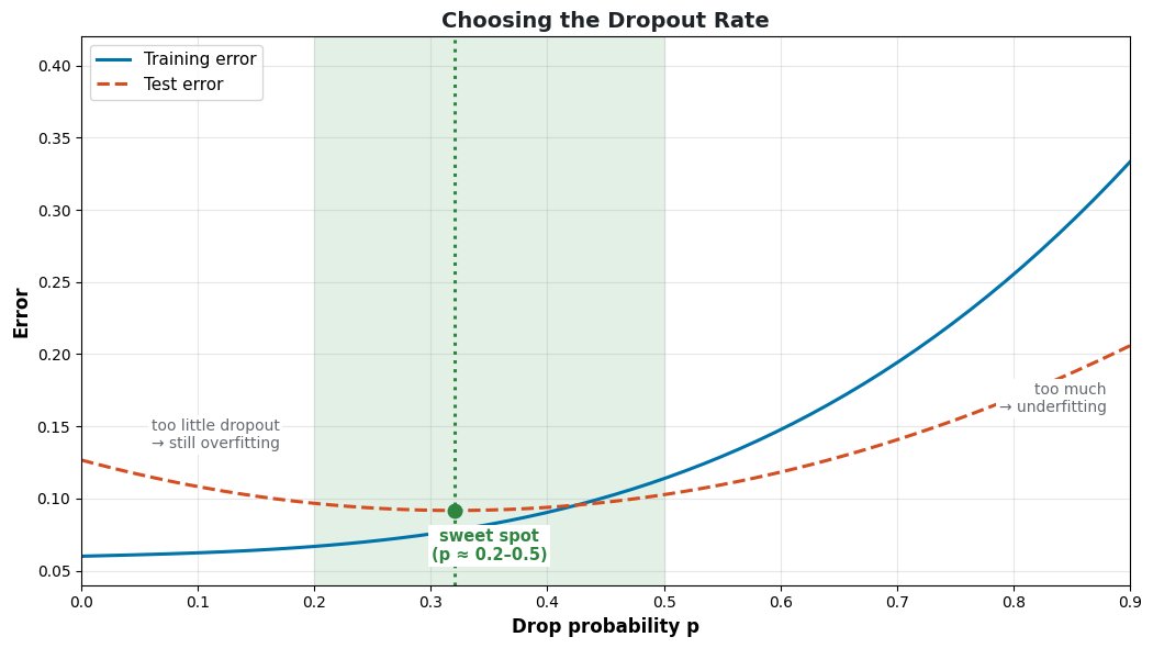
    Training and test error versus dropout rate with a sweet spot region

    Figure 2: Choosing the drop probability p: too little dropout leaves overfitting, too much underfits; the test-error minimum is the sweet spot (typically p around 0.2–0.5).


    Login to view more content