Tag: Transformer

DL0152 VLA Frequency Gap Bridge

How do you bridge the execution frequency gap between a low-frequency VLA policy running at 3 to 10 Hz, as in a pi-0 or GR00T N1 class model, and a high-frequency joint controller demanding 500 to 1000 Hz torque or impedance updates?

Answer

You never let the VLA command joints directly. The frequency gap is closed by a three-tier cascade in which each tier runs at its own clock: the VLA emits an action chunk covering hundreds of milliseconds of future motion instead of a single next action, a mid-rate head or buffer replays that chunk at 20 to 100 Hz, and a real-time layer upsamples the waypoints to the servo rate and closes an impedance or torque loop at 1 kHz against live encoder feedback. Chunking alone is not enough, because a blocking call stalls the controller for the whole inference window, so the chunk is computed asynchronously while the previous one is still executing, and the first few actions of the new chunk are frozen or blended to match what the robot has already committed to. Between waypoints you interpolate with a cubic or minimum-jerk segment rather than holding the last value, since a zero-order hold turns every chunk step into a velocity impulse the drives cannot follow. The real-time layer also owns safety: a watchdog that decays to gravity compensation when the buffer underruns, plus joint limits and torque saturation that the neural policy never sees.

(1) Chunks, Not Single Actions: the policy predicts $H$ future actions per forward pass, converting a 3 to 10 Hz decision rate into a continuous 20 to 100 Hz stream of targets.
(2) Horizon Must Cover Latency: the chunk has to be long enough to keep the buffer fed through one full inference plus transport delay, otherwise execution stutters at every boundary.
(3) Asynchronous Inference: issue the next forward pass while the current chunk still has actions left, so compute overlaps execution instead of interrupting it.
(4) Frozen Prefix And Blending: the first $d$ actions of a fresh chunk are already stale on arrival, so they are discarded or soft-constrained to the committed trajectory to avoid a jump at the splice.
(5) Interpolate, Never Zero-Order Hold: a spline between waypoints spreads each step over the $r$ controller ticks in between and keeps commanded velocity and acceleration bounded.
(6) The 1 kHz Layer Owns Safety: impedance gains, torque limits, and a buffer-underrun watchdog run on a real-time thread that never waits on a GPU.

Vertical three-tier diagram: a VLA backbone at 3 to 10 Hz with 100 to 300 ms inference passes features down to an action expert that emits a chunk of 50 joint targets at 50 Hz, which feeds a real-time layer performing cubic upsampling and a 1 kHz impedance law before reaching the robot joints, with a feedback path returning observations resampled to 5 Hz

Figure 1: Three clocks on one command path. Each tier only has to meet the deadline of the tier below it, so the 200 ms VLA period never appears as a 200 ms hole in the torque loop. Only the bottom tier is hard real time, and it is the only tier that reads encoders at 1 kHz.

The scheduling detail is what separates a demo from a deployed system. In the naive loop you observe, block on the network and the GPU for 100 to 300 ms, then execute the chunk, which means the controller spends a large fraction of every cycle replaying a stale target or holding still, and the robot visibly pauses at each boundary. Running inference asynchronously removes the hole but introduces a second problem: the chunk that arrives at time $t$ was conditioned on the observation from $t - t_{lat}$ , so its early actions describe a state the robot has already left. Real-time chunking handles this by treating the overlap as an inpainting constraint, keeping the first $d$ actions pinned to the trajectory already in flight and letting the sampler adjust only the free tail. The cheaper approximation used by ACT is temporal ensembling: keep every overlapping prediction for the current timestep and average them with weights $w_k = \exp(-mk)$ , which smooths the splice but adds no latency compensation and biases the command toward older observations.

Timing diagram with two lanes: the upper blocking lane alternates 130 ms inference bars with 200 ms execution blocks separated by red hatched 130 ms hold gaps, while the lower asynchronous lane overlaps inference bars with execution so that chunk blocks butt against each other with no gap

Figure 2: With a 130 ms forward pass and a 200 ms chunk, blocking inference leaves the controller starved for 130 ms out of every 330, roughly 39% dead time. Overlapping the next forward pass with the current execution removes the gaps entirely, and the price is that every chunk acts on an observation that is one cycle old, which is exactly what the frozen prefix compensates for.

Mathematical Formulation:
$T_{chunk} = H / f_a$
$d = \lceil f_a \, t_{lat} \rceil$
$H \geq d + \lceil f_a / f_{vla} \rceil$
$r = f_c / f_a$
$\tau = K_p (q_d - q) + K_d (\dot q_d - \dot q) + g(q)$

Where:

$T_{chunk}$ is the wall-clock horizon a single chunk covers, $H$ is the number of actions in the chunk, and $f_a$ is the rate at which those actions are consumed.
$t_{lat}$ is the end-to-end delay from shutter to first usable action, covering encoding, network transport, and the forward pass; $d$ is the resulting number of stale leading actions.
$f_{vla}$ is the policy replan rate, so $\lceil f_a / f_{vla} \rceil$ is how many actions are consumed per replan and the third relation is the no-underrun condition.
$f_c$ is the servo rate and $r$ the upsampling ratio, the number of interpolated setpoints emitted between two consecutive policy waypoints.
$\tau$ is the joint torque, $q_d$ and $\dot q_d$ the interpolated position and velocity setpoints, $q$ and $\dot q$ the measured state, and $g(q)$ the gravity term.
$K_p$ and $K_d$ set the mechanical impedance; low gains make the arm compliant and forgiving of a slightly wrong setpoint, high gains make it track hard and punish every command discontinuity.

Budget For A 5 Hz VLA On A 1 kHz Arm:
$d = \lceil 50 \times 0.13 \rceil = 7$
$\lceil f_a / f_{vla} \rceil = 50 / 5 = 10$
$H \geq 7 + 10 = 17$
$r = 1000 / 50 = 20$

With a 130 ms latency, a 50 Hz action rate, and a replan every 200 ms, the chunk needs at least 17 actions, and shipping $H = 50$ (a 1.0 s horizon) buys margin for a GPU hiccup or a dropped packet. The controller then produces 20 interpolated setpoints per waypoint, so the neural policy is responsible for shape and the real-time layer for smoothness. Note that a longer horizon is not free: everything past the next replan is open-loop motion, so the chunk length trades buffer robustness against reaction time to disturbances, and only the first $f_a / f_{vla}$ actions of a 50-action chunk are normally executed at all.

Two-panel chart: left panel plots a reference joint trajectory against a 5 Hz zero-order-hold staircase, a 5 Hz linear ramp, and a 50 Hz waypoint sequence cubically upsampled to 1 kHz; right panel is a log-scale bar chart of peak commanded joint velocity for the three command paths with a dashed joint velocity limit line

Figure 3: The same intended motion, three command paths. A zero-order hold asks for a finite position jump inside one 1 ms tick, so the implied velocity sits two orders of magnitude above the joint limit and the drive answers with a torque spike. Both interpolated paths stay under the limit, but only the 50 Hz waypoints actually reproduce the reference shape; upsampling a 5 Hz command smooths the command at the cost of cutting the corners of the trajectory.

Property	Blocking chunk + hold	Overlapping chunks + temporal ensembling	Async chunking + frozen prefix
Controller starvation	One dead window per cycle, about 39% duty loss at 130 ms latency	None if the ensemble buffer stays full	None, inference always overlaps execution
Boundary smoothness	Jump whenever the new chunk disagrees with the held target	Smooth, the exponential average filters the disagreement	Smooth by construction, the prefix is pinned to committed actions
Latency compensation	None, the whole chunk is stale by $t_{lat}$	None, and averaging biases toward older observations	Explicit, the first $d$ actions are skipped or constrained
Extra cost	Cheapest, one forward pass per executed chunk	Keeps several chunks in memory, needs a weighting hyperparameter	Needs a client-server split, a chunk buffer, and guided sampling
Reasonable use	Quasi-static pick and place, teleop replay, offline evaluation	On-board policies with low, stable latency	Remote or large models, dynamic tasks, anything with jittery latency

August 19, 2026

DL0151 Diffusion Policy and pi0 Flow Matching

How does Diffusion Policy generate continuous robot action chunks through denoising, and how does Physical Intelligence’s π0 instantiate the same idea as a flow-matching action expert on top of a pretrained vision-language backbone?

Answer

Neither model emits one action per forward pass. Both treat a whole chunk of $H$ future actions as a single high-dimensional sample from a conditional generative model, and they produce it by starting from Gaussian noise and running an iterative sampler conditioned on the current observation. Diffusion Policy does this with a DDPM: a 1D temporal U-Net (or a transformer variant) predicts the noise inside a noisy action sequence, and $K$ denoising steps turn $A^K \sim \mathcal{N}(0, I)$ into an executable chunk, of which only the first $T_a$ actions are executed before replanning. π0 keeps that output object and changes two things. The sampler becomes conditional flow matching along a straight noise-to-action path integrated with about 10 Euler steps, and the denoiser becomes a 300M-parameter action expert placed inside a PaliGemma 3B VLM as a second set of weights in one transformer. Images and language flow through the VLM weights, the robot state and the 50 noisy action tokens flow through the expert weights, and a single shared self-attention operation joins them, which is why the backbone is initialized from a VLM and fine-tuned rather than kept literally frozen.

(1) Chunks, Not Single Actions: the policy models $p(A_t \mid O_t)$ over an $H \times d$ matrix, which suppresses per-step jitter and makes long idle or contact phases survivable.
(2) Denoising Is The Policy: sampling replaces regression, so the network never has to collapse several valid demonstrated behaviors into their average.
(3) Multimodality Is Preserved: an MSE regressor asked to pass left or right of an obstacle outputs the mean of the two, which hits the obstacle; a denoiser draws one mode per rollout.
(4) Receding Horizon Closes The Loop: predict $H$ , execute $T_a \leq H$ , re-observe, resample. This is the only feedback mechanism the chunk has.
(5) Flow Matching Straightens The Path: a linear interpolation between noise and data gives an almost constant velocity field, so 10 integration steps suffice for a 50-step chunk at 50 Hz.
(6) Two Experts, One Attention: π0 routes tokens to modality-specific weights but keeps one attention operation, and the prefix KV cache is computed once per observation while only the small expert runs on every integration step.

Top row shows three line plots of two action dimensions over the fifty steps of a chunk, starting as pure Gaussian noise, then partially denoised, then a smooth executable trajectory, with denoise arrows between them. Bottom panel shows three overlapping horizontal bars representing chunks predicted at successive replanning times, each with a shaded leading segment marking the executed portion.

Figure 1: The sampler operates on the entire chunk at once, so temporal smoothness is a property of the generated sample rather than something enforced by a filter. At the bottom, only the leading $T_a$ actions of each chunk are executed, so the replanning period sets the reaction latency to anything the model did not anticipate.

The reason to pay for an iterative sampler is the shape of the demonstration data. Teleoperated demonstrations are multimodal and idle-heavy: the same scene is solved in several ways, and a maximum-likelihood Gaussian head trained with MSE returns the conditional mean, which is frequently not a valid action. Discretizing each dimension independently avoids averaging but breaks cross-dimension coordination, and a joint discretization is exponential in $d$ . Diffusion Policy’s published recipe uses observation horizon 2, prediction horizon 16, execution horizon 8, 100 DDPM training steps with 10 DDIM inference steps, FiLM conditioning of the observation embedding into a 1D temporal convolutional U-Net, and end-effector position control rather than velocity control, reporting an average 46.9% relative improvement over prior behavior-cloning baselines across 15 tasks.

Diffusion Policy (DDPM formulation):
$A_t = (a_t, a_{t+1}, \ldots, a_{t+H-1})$
$\hat{\epsilon} = \epsilon_{\theta}(O_t, A_t^k, k)$
$A_t^{k-1} = \alpha_k (A_t^k - \gamma_k \hat{\epsilon}) + \sigma_k z$
$\mathcal{L}_{\mathrm{DP}} = \mathbb{E}\|\epsilon - \hat{\epsilon}\|^2$

The same object, an $H \times d$ chunk, is what π0 produces, but the generative process is a continuous-time flow rather than a discrete Markov chain. Training samples a noise vector and a time $\tau \in [0,1]$ from a beta distribution that deliberately over-weights the noisy end of the path, forms the linear interpolant, and regresses the network onto the constant velocity that carries noise to data. Because the path is straight by construction, inference integrates with a fixed step $\delta = 0.1$ from $\tau = 0$ to $\tau = 1$ , which is 10 network evaluations for a chunk of 50 actions at 50 Hz. Cross-embodiment training is handled crudely and effectively: every state and action vector is zero-padded to the largest action dimension in the mixture (18 in the released model), and robots with fewer joints simply ignore the padded slots.

Architecture diagram with four input lanes for camera images, language instruction, robot state, and the noisy action chunk with its tau embedding, each passing through its own encoder into a single transformer stack that contains two weight sets: PaliGemma VLM weights for the prefix tokens and a 300 million parameter action expert for state and action tokens, joined by shared self-attention, producing a velocity field that is integrated by ten Euler steps into the final action chunk.

Figure 2: π0 is a mixture of two experts inside one transformer: the token type decides which weight matrices are applied, while attention is computed jointly over the whole sequence. Only the small expert is re-run per integration step, so the reported cost of a chunk is one 3B prefill plus ten passes over 300M parameters, roughly 73 ms in the released report.

Flow-matching action expert:
$A_t^{\tau} = \tau A_t + (1-\tau)\epsilon$
$u(A_t^{\tau} \mid A_t) = A_t - \epsilon$
$\mathcal{L}_{\mathrm{FM}} = \mathbb{E}\|v_{\theta}(A_t^{\tau}, o_t) - u\|^2$
$A_t^{\tau+\delta} = A_t^{\tau} + \delta\, v_{\theta}(A_t^{\tau}, o_t)$
$H \Delta t = 50 \times 20\ \text{ms} = 1000\ \text{ms}$
$C = C_{\mathrm{VLM}} + 10\, C_{\mathrm{expert}}$

Where:

$A_t \in \mathbb{R}^{H \times d}$ is the action chunk starting at time $t$ , $a_i$ one action, $H$ the prediction horizon (16 in Diffusion Policy, 50 in π0), and $d$ the padded action dimension.
$O_t$ and $o_t$ are the conditioning observations: for Diffusion Policy a short stack of image features and proprioception, for π0 the image tokens, language tokens, and the state token.
$k \in \{K, \ldots, 1\}$ indexes discrete denoising steps and $\epsilon_{\theta}$ is the noise-prediction network; $\alpha_k, \gamma_k, \sigma_k$ come from the noise schedule and $z \sim \mathcal{N}(0, I)$ is the injected sampling noise.
$\tau \in [0,1]$ is the continuous flow time, $\epsilon \sim \mathcal{N}(0, I)$ the noise endpoint, and $A_t^{\tau}$ the linear interpolant between them.
$u$ is the target velocity field of the straight path, $v_{\theta}$ the action expert’s prediction of it, and $\delta = 0.1$ the Euler step, giving 10 evaluations per chunk.
$\Delta t = 20\ \text{ms}$ is the control period at 50 Hz, so one chunk covers one second; $C_{\mathrm{VLM}}$ and $C_{\mathrm{expert}}$ are the per-pass costs of the 3B prefix and the 300M expert.

Three by three block attention matrix with rows as query blocks and columns as key blocks. The prefix row attends only to the prefix column and is marked bidirectional and cached. The state row attends to prefix and state. The action row attends to all three blocks and is bidirectional within the chunk. The remaining upper right cells are hatched as masked.

Figure 3: The blockwise causal mask is what makes the cost structure possible. Because the image and text prefix never attends to the noisy action tokens, its keys and values do not depend on $\tau$ and stay valid across all 10 integration steps, while the action block attends bidirectionally within the chunk so every predicted timestep sees every other.

Property	Diffusion Policy (2023)	π0 (2024)
Generative process	Discrete-time DDPM, epsilon-prediction, cosine or squared-cosine schedule	Continuous-time conditional flow matching on the straight interpolant
Sampler steps	100 training steps, 10 DDIM steps at inference	10 forward Euler steps with fixed step 0.1
Denoiser	1D temporal U-Net with FiLM, or a small transformer variant	300M action expert sharing attention with PaliGemma 3B weights
Conditioning	ResNet image features plus proprioception, no language	Up to 3 camera views, natural-language instruction, state token
Chunk and rate	Predict 16, execute 8, typically about 10 Hz control	Predict 50 actions, one second of control at 50 Hz
Embodiment scope	One robot and task per trained policy	Cross-embodiment mixture, all vectors zero-padded to 18 dimensions
Dominant failure mode	No semantic generalization; the visual encoder is trained from a few hundred demos	Open-loop within a chunk, and prefill latency dominates the control budget

August 19, 2026

DL0150 Generative Multi-View World Model

How do generative world models generate realistic, high-resolution multi-view camera outputs (e.g., 8 ring cameras on a vehicle) with spatial and temporal coherence?

Answer

Modern driving world models are latent video diffusion models rather than per-camera image generators. A causal video tokenizer compresses every camera stream (roughly 16x spatially and 4x temporally), and one diffusion transformer denoises a single latent tensor that holds all 8 views and all frames of the clip simultaneously, so coherence is a property of the sampling process instead of a post-hoc fix. Spatial agreement between neighbouring cameras comes from two ingredients: cross-view attention inside every block, and camera-geometry conditioning that tells each token where its camera points, usually as per-pixel Plücker ray embeddings built from the intrinsics and extrinsics of that rig. Temporal agreement comes from a temporal attention axis plus a shared ego-action and agent-layout condition that all 8 views must obey, so a braking maneuver or a crossing pedestrian appears in every camera at the same instant. High resolution is bought with a cascade instead of brute force: the transformer works in a small latent grid, and a separate diffusion upsampler restores full per-view pixels, while long horizons come from autoregressive rollout over overlapping context frames.

(1) Latent, Not Pixel, Diffusion: a learned video tokenizer removes most spatial and temporal redundancy first, so the generator never denoises 8 megapixel-scale streams directly.
(2) One Joint Tensor Over Views And Time: the state being denoised is $z \in \mathbb{R}^{V \times T \times N \times c}$ , which is why views cannot drift into independent hallucinations.
(3) Factorized 4D Attention: spatial attention within a view-frame, cross-view attention across the ring at a fixed time, and temporal attention across time within a view, roughly 126x cheaper than full joint attention at 8 views and 16 frames.
(4) Geometry As A First-Class Condition: Plücker rays per pixel (plus optional epipolar-constrained attention) let one model serve rigs with different camera counts, mounting positions, and fields of view.
(5) Shared Layout And Action Control: 3D agent boxes, an HD map or BEV raster, and the ego trajectory are broadcast to every view, so all cameras render the same world state rather than eight plausible worlds.
(6) Cascade And Rollout: a super-resolution diffusion stage supplies pixels and an overlapped sliding window supplies duration, at the cost of error accumulation over long horizons.

Pipeline diagram: eight-view video enters a causal video tokenizer with 16x spatial and 4x temporal compression, producing a latent grid of V by T by N tokens that feeds a diffusion transformer of L blocks, then a latent decoder and a diffusion upsampler back to 448 by 960 per view; an expanded panel shows one block containing spatial self-attention within a view-frame, cross-view attention across the eight views at one time step, and temporal attention across frames of one view, with camera Plucker rays, ego action, agent layout, and noise level injected on the right

Figure 1: One tokenizer, one transformer, one upsampler. The only thing that makes this a multi-view model rather than eight video models is the cross-view attention axis and the shared conditioning bundle; the token budget of 215,040 latents per clip is what forces the attention to be factorized.

The cross-view axis is where naive designs fail, and geometry explains why. Ring cameras overlap only with their immediate neighbours, so attending from the rear camera to the front camera buys almost nothing while costing the same as a useful pair; restricting cross-view attention to ring-adjacent views keeps essentially all of the benefit. Inside an adjacent pair, a point visible in view $i$ cannot be anywhere in view $j$ : the fundamental matrix of the calibrated rig confines it to a single epipolar line, which is why epipolar-band attention is a legitimate sparsification rather than a heuristic. Conditioning carries the rest of the load. Because the ego action and the 3D agent boxes are shared, the front-left and front cameras are both being asked to render the same car at the same metric position, and the overlap region then agrees on colour, exposure, geometry, and occlusion because both views were denoised from the same layout under attention that could compare them at every layer.

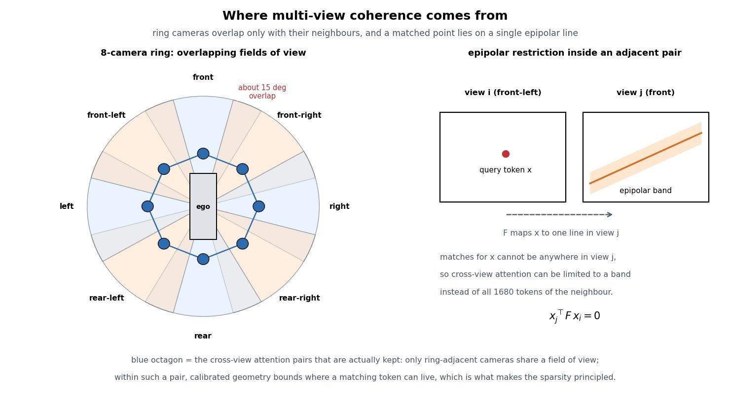
Left panel: top-down view of a vehicle with eight camera field-of-view wedges arranged in a ring, labelled front, front-right, right, rear-right, rear, rear-left, left, and front-left, with a 15 degree overlap marked between neighbours and an octagon of lines connecting adjacent camera nodes to show which pairs exchange cross-view attention. Right panel: two image-plane rectangles for view i and view j, a marked point x in view i and the corresponding epipolar band drawn as a shaded stripe in view j, with the constraint that a matching token lies on that single line.

Figure 2: Coherence is a geometry problem before it is a modelling problem. Only ring-adjacent pairs share a field of view, and within a pair the epipolar constraint bounds where a matching token can live, so both the sparsity pattern and the conditioning signal are dictated by the calibrated rig.

Mathematical Formulation:
$z \in \mathbb{R}^{V \times T \times N \times c}$
$N = (H/p)(W/p) = 28 \times 60 = 1680$
$L = V T N = 8 \times 16 \times 1680 = 215040$
$\mathcal{L}(\theta) = \mathbb{E}\left[\lVert \epsilon - \epsilon_{\theta}(z_t, t, c) \rVert^2\right]$
$c = (r, a, b, z_{\mathrm{ctx}})$
$r_{uv} = (d_{uv},\ o \times d_{uv}) \in \mathbb{R}^{6}$

Where:

$z$ is the joint latent tensor being denoised, with $V=8$ views, $T$ latent frames, $N$ tokens per view-frame, and $c$ latent channels.
$H \times W = 448 \times 960$ is the per-view pixel resolution and $p = 16$ the combined tokenizer and patch downsampling factor, giving a $28 \times 60$ latent map.
$L$ is the total sequence length if the clip were flattened, the number that decides whether full attention is affordable.
$\epsilon$ is the sampled noise, $z_t$ the noised latent at level $t$ , and $\epsilon_{\theta}$ the diffusion transformer.
$c$ bundles the conditioning: per-view rays $r$ , ego action $a$ (speed and curvature), agent and map layout $b$ , and the overlapping context latents $z_{\mathrm{ctx}}$ from the previous window.
$r_{uv}$ is the Plücker embedding of the ray through pixel $(u,v)$ , with unit direction $d_{uv}$ and camera origin $o$ , so extrinsics and intrinsics enter as a 6-channel image instead of a flat vector.

Attention Cost Per Block:
$C_{\mathrm{full}} = L^2 = 4.62 \times 10^{10}$
$C_{\mathrm{spa}} = V T N^2 = 3.61 \times 10^{8}$
$C_{\mathrm{view}} = T N V^2 = 1.72 \times 10^{6}$
$C_{\mathrm{tmp}} = V N T^2 = 3.44 \times 10^{6}$
$C_{\mathrm{spa}} + C_{\mathrm{view}} + C_{\mathrm{tmp}} = 3.66 \times 10^{8}$

Factorization therefore costs about 0.8% of full joint attention at this shape, and almost all of the remaining cost is ordinary within-frame spatial attention. The cross-view and temporal axes together add under 1.5% on top of the spatial term, which is the practical reason multi-view coherence is affordable at all: the expensive part of the model is generating each image, not keeping the images consistent.

Log-scale line chart of attention pairs per transformer block against the number of camera views from 1 to 8, with 16 latent frames and 1680 tokens per view-frame. The full joint 4D attention curve rises quadratically from about 7.2e8 to 4.62e10 pairs, while the factorized spatial plus cross-view plus temporal curve rises nearly linearly from about 2.9e7 to 3.66e8 pairs, an annotation noting the roughly 126x gap at eight views.

Figure 3: Full joint attention over the flattened clip grows as $V^2$ while the factorized form grows close to linearly in $V$ , so the gap widens with every camera added to the rig. Adding a ninth or tenth view is a routine cost in the factorized design and prohibitive in the joint one.

Property	Independent per-view generation	Factorized view + time attention	Full joint 4D attention
Attention pairs per block	3.61e8 (spatial only)	3.66e8, about 1.4% overhead	4.62e10, roughly 126x more
Overlap agreement	None; only the shared layout condition, so seams disagree	Enforced on ring-adjacent pairs, optionally epipolar-banded	Enforced globally, mostly on pairs that never overlap
Temporal behaviour	Per-view only; the eight views desynchronize over rollout	Temporal axis plus one shared action keeps views in lockstep	Strongest in principle, but memory caps the clip length
Failure signature	Objects appear in one camera and vanish in its neighbour	Slow drift of far-field content and appearance across rollout	Out-of-memory or a clip too short to be useful for simulation
Practical verdict	Useless for BEV or occupancy training data	The production choice for ring-camera world models	Research ablation at small resolution or few frames

August 18, 2026

DL0149 World Models from Unlabeled Video

How do world models learn interactive, action-controllable environment rollouts from unlabeled video datasets without ground-truth action labels?

Answer

The missing action labels are invented by the model itself. A latent action model (LAM) is an inverse-dynamics encoder that looks at the past frames and the next frame together and emits a single discrete code $z_t$ through a vector-quantized bottleneck; a forward dynamics model is then required to predict that next frame from the past frames plus $z_t$ alone. Both halves are trained jointly with next-frame reconstruction as the only supervision, so the code is pushed to carry exactly the part of the transition that the past cannot explain, which for gameplay and egocentric video is precisely the agent’s action. Genie made this concrete at scale, training an 11B-parameter model on roughly 30,000 hours of filtered 2D platformer video with a codebook of only $K = 8$ latent actions, and the tiny codebook is not a detail but the mechanism: at 3 bits per step the code physically cannot smuggle the next frame through it. At inference the LAM encoder is thrown away, a key press is mapped onto one of the $K$ learned codes, and the dynamics model rolls the world forward autoregressively, which turns passive video into a playable environment.

(1) Latent Action Model: an inverse-dynamics encoder over $(x_{1:t}, x_{t+1})$ produces one discrete code per transition, standing in for the action label that the dataset never had.
(2) The Bottleneck Is The Whole Trick: a codebook of size $K = 8$ caps the code at $\log_2 8 = 3$ bits, forcing it to describe a control decision rather than pixels.
(3) Reconstruction Is The Only Loss: the forward model’s next-frame error trains the encoder through the quantizer, so no human ever annotates a button.
(4) Tokenize, Then Roll Out: a spatiotemporal VQ-VAE turns frames into tokens and a masked-token or diffusion dynamics model generates the next frame conditioned on the past tokens and $z_t$ .
(5) Codes Are Shared Across Videos: because one codebook serves the whole corpus, the same index means the same intent in unseen scenes, which is what makes the latent space a controller instead of a per-clip artifact.
(6) Grounding To Real Controls Is Cheap: a handful of labeled clips, or human probing of each code, suffices to attach semantics; VPT instead spent 2,000 labeled hours to train an inverse-dynamics model and pseudo-labeled 70,000 web hours with it.
(7) Rollouts Drift: generation is autoregressive on its own output, so compounding error, memory loss, and entangled camera-versus-agent motion dominate the failure list.

Two-panel diagram. The training panel shows past frames and the next frame both entering a latent action model with a VQ bottleneck of eight codes, producing a 3-bit code, while the past frames are separately tokenized by a spatiotemporal VQ-VAE; both streams enter a masked video-token dynamics model whose only loss is reconstruction of the next frame. The inference panel shows a key press selecting one of the eight codes without the latent action model, feeding the same dynamics weights, decoding and rendering a frame that loops back as the next context.

Figure 1: The asymmetry between the two panels is the point. During training the next frame is visible to the latent action model, which is why an unlabeled corpus can supervise a controller; at inference that encoder is discarded and the codebook itself becomes the input device, with the rendered frame fed back as context for the next step.

Everything hinges on how much information the quantizer lets through. If the latent is generous (a wide continuous vector, or a codebook of thousands of entries), the encoder discovers the shortcut of encoding the next frame directly, the dynamics model degenerates into a decoder of the latent, reconstruction looks excellent, and controllability collapses because a user-chosen code no longer corresponds to anything an agent could do. If the latent is too narrow, distinct moves collapse into one code and the environment responds to only a couple of coarse commands. The standard diagnostic is a controllability delta: roll the model forward with the inferred code, then with a random code, and measure the gap in frame quality. A large gap means the code is doing real work; a gap near zero means either leakage or a code the model ignores.

Mathematical Formulation:
$z_t = q(f_{\phi}(x_{1:t+1}))$
$\hat{x}_{t+1} = g_{\theta}(x_{1:t}, z_t)$
$\mathcal{L}(\phi,\theta) = \| x_{t+1} - \hat{x}_{t+1} \|_2^2$
$H(z_t) \leq \log_2 K$
$\Delta = \mathrm{PSNR}(z_t) - \mathrm{PSNR}(\tilde{z})$

Where:

$z_t$ is the latent action for the transition at step $t$ , and $q$ is vector quantization onto a codebook of $K$ entries.
$f_{\phi}$ is the inverse-dynamics encoder, which is the only component allowed to see the future frame, and $\phi$ are its parameters.
$x_{1:t}$ are the observed past frames (in practice their VQ tokens), $x_{t+1}$ is the true next frame, and $\hat{x}_{t+1}$ is the prediction.
$g_{\theta}$ is the forward dynamics model, a masked video-token transformer or a diffusion decoder, conditioned on the past plus $z_t$ and nothing else.
$\mathcal{L}$ is the reconstruction objective, extended in practice by the usual commitment and codebook terms; no action label appears in it, which is why unlabeled video is sufficient.
$H(z_t) \leq \log_2 K$ is the capacity bound that prevents frame leakage, giving 3 bits per step when $K = 8$ .
$\Delta$ is the controllability metric, comparing a rollout driven by the inferred code against one driven by a random code $\tilde{z}$ drawn from the same codebook.

Why 3 Bits Cannot Encode A Frame:
$\log_2 K = \log_2 8 = 3 \ \text{bits}$
$256 \times 10 = 2560 \ \text{bits per frame}$

A $16 \times 16$ token grid over a 1024-entry visual codebook already carries about 2,560 bits, roughly three orders of magnitude more than the action code, so the encoder has no route to cheat and the dynamics model must genuinely keep a model of the scene in its context. That ratio is the design knob you actually tune: too small and the environment is unresponsive, too large and it stops being an environment at all.

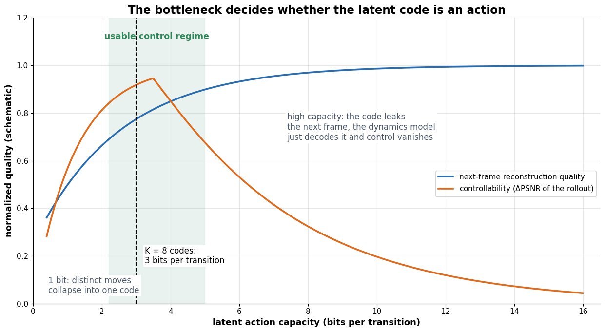
Schematic line chart with latent action capacity in bits per transition on the x-axis and normalized quality on the y-axis. Next-frame reconstruction quality rises monotonically and saturates, while controllability rises to a peak near three bits and then decays toward zero as capacity grows, with a shaded band marking the usable control regime between about two and five bits and a dashed vertical line at three bits labeled as an eight-entry codebook.

Figure 2: Schematic view of the tension that a single reconstruction loss hides. Reconstruction quality never warns you about failure because it keeps improving as the latent widens, whereas controllability peaks and then collapses once the code can carry the frame; only the two curves together tell you the bottleneck is set correctly.

Property	Latent action model (no labels)	Inverse-dynamics pseudo-labeling	Logged true actions
Label requirement	None during training; a few clips only to name the codes	A labeled seed set, such as VPT’s 2,000 contractor hours	Every frame paired with the true control input
Action space	Discovered discrete codes, semantics unknown a priori	The real action API, recovered by a trained predictor	The real action API, exactly
Data ceiling	Any internet video of the domain	Any video, but the seed set must match the domain	Only instrumented environments and agents
Dominant failure mode	Frame leakage through a wide latent, or codes entangling camera and agent motion	Pseudo-label noise on rare actions propagates into the dynamics	Coverage limited to the logging policy’s behaviour
Representative system	Genie, LAPO	VPT	GameNGen, Dreamer-style agents

August 18, 2026

DL0148 Action Chunking Transformer (ACT)

Explain the Action Chunking Transformer (ACT). How does predicting sequences of future action vectors ( $k$ -step horizons) solve temporal inconsistency and compounding error drift?

Answer

ACT is the imitation-learning policy introduced with the ALOHA bimanual setup: a transformer encoder-decoder that takes the current multi-view images plus the 14-dimensional joint state and emits, in a single forward pass, a whole chunk of $k=100$ future joint-position targets rather than one action. It is trained as a conditional VAE (CVAE) with an $L_1$ reconstruction loss on the chunk plus a KL term on a small style latent $z$ , which lets one deterministic-at-test-time policy absorb the multimodality of human teleoperation instead of averaging it away. Chunking attacks drift arithmetically: at 50 Hz a 20-second task is 1,000 control steps but only $1000/100 = 10$ chunk decisions, so the number of places where the policy can leave the training distribution shrinks by a factor of $k$ and the classic $O(\epsilon T^2)$ behaviour-cloning bound falls to roughly $O(\epsilon T^2 / k)$ . Chunking also removes per-step temporal inconsistency, because the actions inside a chunk are generated jointly from one latent and one observation, so the policy cannot flip between two valid modes on consecutive 20 ms steps. To avoid a visible discontinuity when a new chunk starts, ACT still queries the network every step and blends the overlapping predictions with temporal ensembling.

(1) The Chunk Is The Output Unit: the policy models $\pi(a_{t:t+k-1} \mid o_t)$ instead of $\pi(a_t \mid o_t)$ , so $k$ correlated actions are predicted together as one object.
(2) Effective Horizon Divided By $k$ : the agent makes $H = \lceil T/k \rceil$ sequential decisions, and compounding error grows with the number of decisions, not with the number of motor commands.
(3) CVAE For Multimodality: a BERT-style encoder compresses the demonstrated chunk into a 32-dimensional latent $z$ during training and is discarded at test time, where $z = 0$ gives one clean decisive mode.
(4) Non-Markovian Demos Stop Being Fatal: a single-step policy standing at a human pause sees a bimodal target (hold still or move) and can freeze forever; a chunk that contains the pause and the following motion resolves the ambiguity.
(5) Temporal Ensembling For Smoothness: re-query every step and average the overlapping chunk predictions with weights $w_i = \exp(-m i)$ , which keeps reaction latency at one control step while removing chunk-boundary jumps.
(6) $L_1$ Over $L_2$ : the $L_1$ loss on absolute joint targets produces sharper, less smeared trajectories, which matters for millimetre-scale contact tasks.

Architecturally there is nothing exotic. Each of the four RGB streams (two wrist cameras, two static cameras at 480×640) goes through a ResNet-18 whose final feature map is flattened into roughly 300 tokens, the joint vector becomes one more token, and the style latent becomes one more; a 4-layer transformer encoder with width 512 mixes them, and a 7-layer decoder attends to that memory from $k$ fixed learned position embeddings, one per future step, so the $k \times 14$ output is produced non-autoregressively in about 0.01 s. The whole policy is roughly 80M parameters trained from scratch per task on about 50 demonstrations, which is the interesting part: the gain does not come from scale or pretraining, it comes from changing what a single prediction means.

Architecture diagram of ACT: four RGB cameras feed per-camera ResNet-18 backbones producing about 300 tokens each, a joint-position token joins them, a 4-layer transformer encoder mixes the tokens, a 7-layer decoder with k learned queries emits a k by 14 action chunk, and above the main lane a training-only CVAE encoder maps the demonstrated action sequence and joint state to a 32-dimensional style latent z that is injected into the encoder and set to zero at test time

Figure 1: ACT is a CVAE whose decoder is a chunk predictor. The dashed lane exists only during training: it sees the ground-truth action sequence and squeezes the demonstrator’s stylistic choice into $z \in \mathbb{R}^{32}$ . At test time $z$ is fixed to the prior mean, so the same network becomes a deterministic policy that outputs $k \times 14$ absolute joint targets in one pass.

Mathematical Formulation:
$\pi_\theta(\hat a_{t:t+k-1} \mid o_t, q_t, z)$
$\mathcal{L}_1 = \sum_{j=0}^{k-1} \| \hat a_{t+j} - a_{t+j} \|_1$
$\mathcal{L} = \mathcal{L}_1 + \beta \, D_{\mathrm{KL}}(q_\phi \, \| \, \mathcal{N}(0, I))$

Where:

$\hat a_{t:t+k-1}$ is the predicted action chunk, here $k=100$ absolute target joint configurations in $\mathbb{R}^{14}$ for a bimanual 6-DoF-plus-gripper arm pair.
$o_t$ are the four camera images at time $t$ and $q_t$ the measured joint positions, together forming the only observation the chunk is conditioned on.
$z \in \mathbb{R}^{32}$ is the style latent, sampled from the encoder posterior $q_\phi(z \mid a_{t:t+k-1}, q_t)$ in training and set to $z = 0$ at inference.
$j \in \{0, \ldots, k-1\}$ indexes positions inside the chunk, each produced by its own learned decoder query.
$\beta$ weights the KL term; a large $\beta$ collapses $z$ to noise while a small one lets the encoder leak the answer and hurts test-time behaviour.
The $L_1$ norm is deliberate: it penalises large joint errors less quadratically than $L_2$ and therefore averages competing modes less aggressively.

The drift argument is worth writing down. Standard behaviour cloning with per-step error $\epsilon$ suffers covariate shift: a mistake moves the robot to a state the demonstrations never covered, the next prediction is worse, and the regret bound is quadratic in the horizon. Chunking does not make the policy immune, it reduces how many times the loop is closed. With $H = T/k$ decision points, each contributing error $\epsilon$ that persists over the remaining decisions, and each decision covering $k$ timesteps of cost, the accumulated term scales as $\epsilon H^2 k = \epsilon T^2 / k$ . The same factor cuts inference calls, which is why a chunked policy can afford a much heavier network per decision.

Horizon Arithmetic At 50 Hz:
$T = 20 \times 50 = 1000$
$H = \lceil 1000 / 100 \rceil = 10$
$\mathcal{E}_{\mathrm{BC}} = O(\epsilon T^2)$
$\mathcal{E}_{\mathrm{chunk}} = O(\epsilon T^2 / k)$

Semi-log chart of a compounding-error bound scale against episode length in control steps at 50 Hz, with three parabolic curves for chunk size k equal to 1, 10, and 100, showing the k equals 100 curve two orders of magnitude below the single-step curve, annotated with the point where a 20 second task of 1000 steps requires only 10 chunk decisions

Figure 2: The bound is still quadratic in task length, so chunking does not abolish drift, it buys two orders of magnitude at $k=100$ . The practical reading is that a long-horizon task becomes as hard as a short one only if the chunk itself remains executable open-loop, which is exactly the assumption that breaks when the scene moves during the 2 seconds a chunk spans.

Naive open-loop execution of the chunk creates a new problem: every 2 seconds a fresh observation produces a fresh chunk that need not start where the previous one ended, and the robot jerks. ACT therefore runs the policy at the full control rate and aggregates. At timestep $t$ there are up to $k$ different chunks that predict an action for $t$ , one from each of the previous $k$ queries, and the executed command is their exponentially weighted mean with $m = 0.01$ , where index $i = 0$ is the oldest prediction. That value of $m$ keeps the weights nearly uniform (1.00, 0.99, 0.98, …), so new observations are folded in immediately while the average stays smooth; a larger $m$ leans on the oldest chunk and reacts more slowly.

Temporal Ensembling:
$w_i = \exp(-m i)$
$\bar a_t = \sum_i w_i \hat a_t^{(i)} / \sum_i w_i$

Timeline diagram with four horizontal rows of six cells each, one row per chunk issued at timesteps 0, 1, 2 and 3, staggered so that all four rows cover timestep 4; the four cells covering timestep 4 are highlighted and labelled with exponential weights 1.00, 0.99, 0.98 and 0.97, and an arrow leads down to a box stating that the executed action at timestep 4 is the weighted mean of the four overlapping predictions

Figure 3: Chunks overlap because the policy is queried every step, so each control command is a vote of up to $k$ predictions made from $k$ different observations. This is what keeps ACT closed-loop at 50 Hz while its prediction horizon stays 2 seconds long, and it costs one extra forward pass per step rather than any extra training.

Property	Single-step BC (k = 1)	Chunk, open-loop execution	ACT: chunk + temporal ensembling
Policy output	One 14-d joint target	100 x 14 targets, all executed	100 x 14 targets, blended with earlier chunks
Queries per 20 s task	1,000	10	1,000 (each cheap, 0.01 s)
Decision points that can drift	1,000, bound scales as eps T^2	10, bound scales as eps T^2 / k	10 committed motions, continuously re-averaged
Reaction to a disturbance	20 ms	Up to 2 s of stale commands	20 ms, damped by the weighted mean
Human pauses in demos	Bimodal target, policy can freeze	Pause is inside the chunk, resolved	Same, plus no boundary discontinuity
Dominant failure	Jitter and mode switching between steps	Jerk at chunk boundaries, blindness mid-chunk	Averaging across modes can blur a decisive motion

August 18, 2026

DL0147 Multi-Task VLA Negative Transfer

How do multi-task VLA policies, such as the RT-X models trained on the Open X-Embodiment dataset, avoid negative task transfer when trained across heterogeneous robot arms, grippers, and kinematic chains?

Answer

Negative transfer in a cross-embodiment VLA is not a mysterious optimization pathology; it is the direct consequence of the same observation-instruction pair mapping to different correct action vectors on different robots, so the per-embodiment gradients on shared weights partially cancel. The fix is to decide, layer by layer, what genuinely transfers and what does not: vision-language grounding transfers and stays fully shared, while action semantics do not and are pushed into a canonical action space plus embodiment-specific output parameters. In practice that means four moves applied together: canonicalize actions into a common frame with per-dataset percentile normalization, condition the policy on an explicit embodiment token so the target is identifiable, decode through a per-embodiment head or a padded action expert so incompatible outputs never share a final linear layer, and control the data mixture so one 100k-episode domain does not dominate the average gradient. Only after those are in place is gradient surgery (PCGrad, CAGrad) worth its cost, because most measured conflict in early cross-embodiment runs comes from unnormalized, mis-framed action labels rather than from a real task disagreement.

(1) Shared Trunk, Split Output: the ViT plus language backbone sees every dataset, and all embodiment-specific incompatibility is confined to the last block, which is where the conflicting gradients would otherwise meet.
(2) Canonical Action Space: relative end-effector deltas in a fixed camera or base frame, with a normalized gripper channel, make “move 2 cm right” mean the same thing on a Franka and a WidowX.
(3) Per-Dimension Percentile Normalization: mapping each action dimension by its 1st and 99th dataset percentiles into $[-1,1]$ removes the scale mismatch between a 0.08 m gripper stroke and a 0.03 m one.
(4) Explicit Embodiment Conditioning: an embodiment id, proprioceptive state, and control-rate token make the label identifiable; without them the policy is asked to regress a multi-modal target from an ambiguous input.
(5) Mixture Weighting And Capacity: per-domain sampling caps stop large datasets from monopolizing updates, and added capacity (more parameters, or modality/embodiment-aware routing) converts interference into specialization.
(6) Measure Conflict Before Fixing It: log pairwise gradient cosine similarity between embodiment groups and per-domain validation loss, then apply projection methods only to the pairs that are genuinely negative.

The heterogeneity is concrete rather than abstract. A 7-DoF arm commanded in end-effector deltas at 3 Hz, a 6-DoF arm commanded in joint velocities at 5 Hz, and a 14-DoF bimanual rig commanded in absolute joint positions at 50 Hz produce label vectors of different dimension, unit, frame, and scale. Stack them into one tensor and regress with one output layer, and that layer must fit a multi-modal conditional distribution whose modes are mutually contradictory, so the mean-seeking L1 or MSE solution is a blurred command that satisfies nobody. The RT-X study made the asymmetry visible: the small 35M-parameter policy gained substantially on data-poor domains while losing to the original single-domain policies on some data-rich ones, whereas the far larger vision-language-backboned variant did not, which is the classic capacity-limited interference signature. Action chunking makes the stakes higher still, because a head predicting a horizon of $H$ steps outputs $H \times d_a$ numbers whose meaning is embodiment-dependent at every position.

Architecture diagram with three input boxes for RGB observations, the language instruction, and an embodiment id plus proprioceptive spec, all feeding one tall shared vision-language trunk, which produces a shared latent that fans out to three separate action heads for a 7-DoF arm at 3 Hz, a 14-DoF bimanual rig at 50 Hz, and an 8-DoF mobile manipulator, each emitting an action vector of different dimension

Figure 1: Where heterogeneity is absorbed. Everything to the left of the latent is shared across every robot and is exactly the part that benefits from pooled data; everything to the right is embodiment-specific, so a 14-DoF joint-position label and a 7-DoF end-effector delta label never contend for the same output weights. The embodiment id enters as a token in the trunk and also selects the head.

Mathematical Formulation:
$z = f_{\theta}(o_{1:n}, \ell, c_e)$
$\hat{a} = h_{\phi_e}(z)$
$\mathcal{L}(\theta, \phi) = \sum_{e=1}^{E} w_e \mathcal{L}_e$
$g_e = \nabla_{\theta} \mathcal{L}_e$
$\cos(g_i, g_j) = \frac{g_i^{\top} g_j}{\lVert g_i \rVert \lVert g_j \rVert}$
$g_i' = g_i - \frac{g_i^{\top} g_j}{\lVert g_j \rVert^2} g_j$

Where:

$z$ is the shared latent produced by the trunk $f_{\theta}$ from the camera views $o_{1:n}$ , the instruction $\ell$ , and the embodiment context $c_e$ (robot id, proprioceptive state, control rate).
$h_{\phi_e}$ is the head for embodiment group $e$ , with its own output dimension $d_a^{(e)}$ and chunk horizon, so $\hat{a} \in \mathbb{R}^{H \times d_a^{(e)}}$ .
$w_e$ are the mixture weights over $E$ embodiment groups, set by capped sampling rather than raw episode counts, and $\mathcal{L}_e$ is the behaviour-cloning loss on group $e$ .
$g_e$ is that group’s gradient with respect to the shared parameters only; head parameters $\phi_e$ receive gradient from one group and cannot conflict by construction.
The cosine is the diagnostic: a negative value means the two groups disagree about the shared update, and its magnitude tells you how much of each step is being cancelled.
$g_i'$ is the PCGrad projection of $g_i$ onto the normal plane of $g_j$ , applied only when the cosine is negative and symmetrically for $g_j'$ .

Per-Dimension Action Normalization:
$\tilde{a}^{(d)} = 2 \frac{a^{(d)} - q_{1}^{(d)}}{q_{99}^{(d)} - q_{1}^{(d)}} - 1$

Percentiles rather than min-max are used because teleoperation logs contain jitter spikes that would otherwise compress the useful range into a few percent of the interval. Note also what normalization cannot repair: it aligns scales, not semantics. If one dataset logs joint velocities and another logs end-effector deltas, both normalized to $[-1,1]$ , the shared head still sees two incompatible meanings for the same slot, which is precisely the residual conflict that per-embodiment decoding removes.

Two-panel vector diagram in the plane. Left panel shows a bimanual gradient pointing up and a single-arm gradient pointing down-left with an angle of about 117 degrees between them, and their sum drawn as a short vector, illustrating cancellation. Right panel shows the same two gradients as faint dashed arrows plus their PCGrad projections drawn solid, whose sum is a longer vector that still descends both losses

Figure 2: Negative transfer, geometrically. When two embodiment groups have gradient cosine near -0.45, their raw sum is shorter than either gradient, so the shared trunk barely moves while both per-domain losses stall. After projecting each gradient onto the other’s normal plane, the combined step is longer and its inner product with both original gradients stays positive, which is the formal statement of “descends both tasks”.

Choosing where the embodiment-specific parameters live is the main design decision, and three families are in use. A single padded head defines one action vector of maximum width and zero-pads unused dimensions, with the loss masked over the padding, which keeps the model monolithic and transfers well when the padded dimensions are physically comparable. Per-embodiment heads require no cross-robot alignment at all and are the most robust to genuinely different control interfaces, at the cost of one head per group and no head for an unseen robot. Latent action spaces learn a discrete or continuous code from video by inverse dynamics, train the policy in that code, and attach a small decoder per robot, which unlocks human video and action-free data but adds an entire quantization stage that can lose fine-grained precision.

Property	Single padded head	Per-embodiment heads	Latent action space
How heterogeneity is handled	One max-width action vector, unused slots zero-padded and masked in the loss	One output module per action space, no alignment across robots needed	Policy predicts a robot-agnostic code, small per-robot decoder maps it to motors
Negative-transfer risk	Moderate: slots must be semantically comparable or the head averages modes	Lowest at the output layer, residual conflict only in the shared trunk	Low if the code is truly embodiment-invariant, high if it leaks robot identity
Unseen robot at test time	Works if its dimensions fit the padded layout	Needs a new head plus a short fine-tune on target data	Needs only a cheap decoder, which is the main selling point
Extra cost	Wasted output width and careful mask bookkeeping	Linear growth in heads, and per-group data must be sufficient	A separate latent-action pretraining stage and possible precision loss
Representative systems	Flow-matching action experts with padded dimensions, unified-action diffusion policies	Readout-head generalist policies and cross-embodied transformers spanning manipulation and navigation	Latent-action pretraining from human and web video

August 18, 2026

DL0146 VLA Continuous Action Representation

How does a transformer decoder represent multi-modal continuous robot actions (e.g., 7-DoF arm pose, gripper state, base velocity) alongside language tokens, as in Google’s RT-2 and the OpenVLA models?

Answer

The decoder never sees a float. Heterogeneous degrees of freedom are first concatenated into one fixed-width vector (end-effector deltas in metres and radians, a gripper command, base velocities, and a discrete mode flag that says which sub-system is being driven this step), then each dimension is independently normalized by its own 1st and 99th percentile statistics so that metres, radians, and a binary gripper all live on $[-1, 1]$ . In the RT-2 and OpenVLA line each normalized dimension is uniformly discretized into 256 bins and the bin index is mapped onto reserved token ids, typically the 256 least-frequently-used entries of the existing SentencePiece or Llama vocabulary, so an action literally becomes a short string of tokens appended to the same causal sequence that holds the image patches and the instruction. Nothing about the architecture changes: the same causal self-attention, the same softmax, and the same cross-entropy loss that predict the next sub-word now predict the next joint delta, which is exactly what lets a VLA inherit internet-scale pretraining. The cost is a quantization floor plus one sequential decoder step per degree of freedom, which is why newer systems keep the shared prefix but replace the discrete head with a continuous action expert that emits a whole chunk of future actions through diffusion or flow matching in a single pass.

(1) One Flat Vector, Fixed Slots: arm, gripper, and base share a single $D$ -dimensional action vector with fixed slot semantics, and unused slots are zero-padded so one model can serve several embodiments.
(2) A Mode Dimension, Not Separate Heads: RT-1 carries an explicit mode variable that switches between controlling the arm, controlling the base, and terminating the episode, so mutually exclusive sub-spaces are disambiguated inside the same vector.
(3) Per-Dimension Quantile Normalization: statistics are computed per dimension and per dataset, using percentiles rather than min and max, because a handful of teleoperation jerks would otherwise consume most of the dynamic range.
(4) 256 Bins Onto Reserved Vocabulary Ids: the action alphabet is carved out of the language vocabulary, so no new embedding table, output head, or loss function is introduced.
(5) Autoregressive Factorization Across DoFs: the chain rule over dimensions lets the yaw bin depend on the already-emitted $x$ and $y$ bins, which is what keeps the joint action coherent rather than per-axis independent.
(6) Action Chunking And Continuous Heads: predicting $H$ future steps at once fights compounding error and raises the effective control rate, and a flow-matching expert removes the bin grid entirely at the price of extra weights and solver steps.

Architecture diagram showing camera frames, instruction text, and proprioception each tokenized into a shared prefix sequence feeding a decoder-only transformer, which branches into a discrete head that emits 256-bin indices as reserved vocabulary tokens and a continuous action expert that emits an H by D chunk by flow matching, both producing the same 11-dimensional action vector of six arm deltas, one gripper command, three base velocities, and one mode flag

Figure 1: The prefix is modality-agnostic; only the head differs. The discrete head reuses the language softmax and spends one sequential decoder step per degree of freedom, while the continuous action expert attends to the same prefix but emits an entire $H \times D$ chunk of real numbers. Both write into the identical fixed-slot action vector, including the mode flag that selects arm, base, or episode termination.

Normalization is where most of the real accuracy is won or lost, and it is the step engineers most often get wrong. Raw teleoperation logs are heavy-tailed: a few reset motions or dropped-controller frames produce end-effector deltas an order of magnitude larger than anything the policy needs at test time. If the bin edges are set by the observed minimum and maximum, those rare samples stretch the grid so far that the entire working range of the robot collapses into a few dozen of the 256 available levels, and the policy inherits a positional resolution floor of several millimetres that no amount of extra data can fix. Clipping to the 1st and 99th percentile before binning, as OpenVLA does, spends the full alphabet on the range the robot actually operates in and pushes the residual error below the mechanical repeatability of most arms. The same argument applies to the gripper, which is near-binary in the data, so it is usually thresholded into open or closed rather than treated as a smooth continuous axis.

Two histograms of the same end-effector delta-z distribution. The left panel bins over the raw min-max range, where rare large outliers stretch the grid and only a small fraction of the 256 bins are ever occupied. The right panel clips to the 1st and 99th percentile before binning, and nearly all 256 bins are occupied with a much smaller bin width in millimetres.

Figure 2: The same action dimension, two bin grids. Min-max binning lets rare teleoperation outliers dictate the grid, so most of the 256 levels are never used and the effective step size is coarse. Quantile binning throws away 2% of the samples and buys back an order of magnitude in resolution per bin, which is why percentile statistics are standard in production VLA data pipelines.

Mathematical Formulation:
$a_t = (a^{\mathrm{arm}}_t, a^{\mathrm{grip}}_t, a^{\mathrm{base}}_t, m_t)$
$\tilde{a}_i = \mathrm{clip}(a_i, q^{i}_{1}, q^{i}_{99})$
$u_i = 2 (\tilde{a}_i - q^{i}_{1}) / (q^{i}_{99} - q^{i}_{1}) - 1$
$b_i = \lfloor 255 (u_i + 1) / 2 \rfloor$
$\mathrm{id}_i = V - 1 - b_i$
$p(a_t \mid c) = \prod_{i=1}^{D} p(b_i \mid c, b_{1:i-1})$

Where:

$a_t$ is the action at control step $t$ , built from an arm delta pose (three translations and three rotations), a gripper command, a base velocity triple, and a discrete mode flag $m_t$ .
$a_i$ is the raw value of dimension $i$ and $\tilde{a}_i$ its clipped version; $q^{i}_{1}$ and $q^{i}_{99}$ are the per-dimension percentiles estimated on the training corpus.
$u_i \in [-1, 1]$ is the normalized value and $b_i \in \{0, \ldots, 255\}$ the bin index, so the grid holds 256 levels per dimension.
$V$ is the language vocabulary size, and $\mathrm{id}_i$ overwrites the 256 least-used token ids at the tail of that vocabulary.
$c$ is the prefix (image patch tokens, instruction sub-words, optional proprioception) and $i \in \{1, \ldots, D\}$ indexes the action dimensions in a fixed canonical order.
The product is the autoregressive factorization: each bin is conditioned on all previously emitted bins of the same action, so the joint distribution is not a product of independent marginals.

Resolution And Token Budget:
$\Delta_i = (q^{i}_{99} - q^{i}_{1}) / 256$
$\Delta = 0.1\ \mathrm{m} / 256 \approx 0.39\ \mathrm{mm}$
$N = H \times D = 8 \times 11 = 88$

Those two lines set the entire engineering trade-off. A translation axis clipped to $\pm 0.05$ m resolves to about 0.39 mm per bin, which is fine for pick and place and marginal for connector insertion, but an eight-step chunk of an 11-dimensional action costs 88 sequential decoder passes, which caps a 7B VLA at roughly 3 to 10 Hz on a single accelerator. The alternative keeps the shared prefix and attaches a small action expert whose tokens are continuous rather than discrete: starting from noise, it integrates a learned velocity field for a handful of solver steps and emits the whole chunk at once, which is how flow-matching policies reach 50 Hz dexterous control. Crucially, both the categorical head and the flow head are distributional, and that matters more than resolution: when two different behaviours are equally valid, a plain L2 or Gaussian regression head averages them into an action that belongs to neither mode.

$A_t = (a_t, a_{t+1}, \ldots, a_{t+H-1})$
$A^{\tau + \delta} = A^{\tau} + \delta\, v_{\theta}(A^{\tau}, \tau, c)$

Left panel shows a top-down workspace with an obstacle and two valid detour trajectories, one above and one below, plus a straight-line mean trajectory that drives into the obstacle. Right panel shows a bimodal action density with a 256-way softmax step approximation covering both peaks and a red dashed vertical line marking the L2 optimum located in the empty valley between the modes.

Figure 3: Why the head must be distributional. Two demonstrators route around the same obstacle in opposite directions, so the conditional action distribution is bimodal; a regression head minimizing L2 lands on the mean, which is a collision. A 256-way categorical over bins, or a diffusion or flow head over the chunk, keeps both peaks and samples one of them.

Property	Discrete bins as vocabulary tokens	Diffusion / flow action expert	Direct continuous regression
Output form	256-way categorical per DoF over reserved token ids	Real-valued chunk of shape H by D, denoised from noise	One real vector, the predicted mean action
Training objective	Cross-entropy, identical to language pretraining	Flow-matching or denoising regression on noised chunks	L2 or L1 on the action vector
Cost per chunk	H times D sequential decoder steps (88 at H=8, D=11)	One prefix pass plus about 10 solver steps of a small expert	One forward pass
Multimodal actions	Yes, per-DoF peaks are tied together by the chain rule	Yes, jointly over the whole chunk	No, collapses to the mean
Resolution	Bin width, about 0.39 mm on a 0.1 m range	Continuous, limited only by data noise	Continuous
Dominant failure mode	Quantization floor plus slow autoregressive decoding	Extra weights and solver steps, harder to co-train with text	Mode averaging produces an invalid middle action

August 18, 2026

DL0145 ITC, ITM, and MLM Pretraining Losses

Compare Image-Text Contrastive (ITC), Image-Text Matching (ITM), and Masked Language Modeling (MLM) losses used in foundational vision-language pre-training, as in models like OpenAI’s CLIP and Salesforce’s BLIP.

Answer

The three objectives differ along three axes: how much cross-modal interaction they permit, which parameters receive gradient, and what the pretrained model can actually do afterwards. ITC is a dual-encoder loss that compresses each image and each caption into a single L2-normalized vector and maximizes the cosine similarity of matched pairs against the other pairs in the batch, so it produces embeddings that can be precomputed and indexed, at the price of never letting a word look at a patch. ITM is a cross-encoder loss: image and text tokens are fused with cross-attention and a binary head decides match or no-match, which gives token-level discrimination but requires one joint forward pass per candidate pair, so it can only ever be a reranker. MLM masks about 15% of the text tokens and reconstructs them conditioned on the image, which is the objective that forces word-to-region grounding and trains the language head that downstream VQA and captioning heads reuse. CLIP trains ITC alone at batch 32,768; ALBEF and BLIP train all three at equal weight because each one supplies something the others cannot.

(1) ITC Learns Global Alignment: an InfoNCE objective over the $N \times N$ in-batch similarity matrix, with $N-1$ negatives per anchor and a learned temperature, optimized symmetrically image-to-text and text-to-image.
(2) ITM Learns Fine-Grained Verification: binary cross-entropy on the fused $\mathrm{[CLS]}$ state, and it is nearly useless unless the negatives are hard negatives mined from the ITC similarity distribution.
(3) MLM Learns Grounded Language: reconstructing masked words from surrounding text plus image evidence ties nouns and attributes to specific patches and yields a vocabulary-sized output head that pure ITC models do not have.
(4) Different Architectural Footprint: ITC updates only the two unimodal towers and their projections, while ITM and MLM update the cross-attention fusion layers; only ITC leaves behind vectors you can put in an ANN index.
(5) Different Compute Profile: ITC is one forward pass per modality but needs a huge batch or a momentum queue (65,536 in ALBEF), whereas ITM and MLM add fusion passes, so BLIP runs its text stack three times per step.
(6) They Compose Into A Pipeline: ITC → hard-negative mining → ITM rerank is the standard retrieval stack, and MLM is the branch that makes the same weights usable for generation-flavored tasks.

Three side-by-side computation graphs. The ITC panel shows separate image and text encoders feeding L2-normalized projections, then an N by N similarity matrix, then an InfoNCE loss. The ITM panel shows both encoders feeding cross-attention fusion layers, then a joint CLS hidden state, then a two-way match versus no-match head using hard negatives. The MLM panel shows the image encoder and a text stream with 15 percent of tokens masked feeding the same fusion layers, then hidden states at masked positions, then a softmax over a 30k word-piece vocabulary.

Figure 1: The same two towers, three different graphs. ITC stops at a single pooled vector per modality, so no gradient ever reaches a fusion layer; ITM and MLM share the cross-attention stack and differ only in the head placed on top, which is why adding MLM to an ITM model is cheap while adding either to a CLIP-style model requires new parameters.

The three losses are not interchangeable because they fail in different directions. An ITC-only model scores “a man in a red shirt riding a bike” and “a man in a blue shirt riding a bike” almost identically, since a single 512-dimensional vector cannot preserve every attribute binding; this is the classic bag-of-words behavior that compositionality benchmarks expose. ITM fixes exactly that case because the fused representation can compare the color word against the actual patches, but its cost is $O(NM)$ joint forward passes for a gallery of $N$ images and $M$ captions, which is why ALBEF and BLIP use ITC to shortlist $k$ candidates and only then run ITM. MLM contributes something neither of the other two does: because the target is a token id rather than a pair label, it forces the model to represent which region licenses which word, and it produces the token-level head that VQA fine-tuning reuses. The coupling runs the other way too, since the ITM negative sampler reads its distribution from the ITC matrix, so a weak ITC head starves ITM of informative negatives.

Left panel: an eight by eight grayscale similarity matrix for one batch, with bright diagonal cells outlined in blue as positive pairs and one bright off-diagonal cell at image four versus text seven outlined in red as the hardest negative. Right panel: a bar chart of the softmax distribution over the eight texts for image four, with a tall blue bar for the true caption, a nearly as tall red bar for the hard negative, and six short gray bars for the easy negatives.

Figure 2: One batch, two uses of one matrix. ITC consumes the whole row and the whole column as a softmax classification problem, while ITM samples a single off-diagonal entry with high similarity and feeds that pair to the fusion encoder labelled no-match. The six near-zero bars are the reason random negatives teach ITM almost nothing: the easy cases already carry negligible gradient.

Mathematical Formulation:
$s_{ij} = z_i^{\top} t_j / \tau$
$\mathcal{L}_{\mathrm{i2t}} = -\log \frac{\exp(s_{ii})}{\sum_{j} \exp(s_{ij})}$
$\mathcal{L}_{\mathrm{itc}} = \tfrac{1}{2}(\mathcal{L}_{\mathrm{i2t}} + \mathcal{L}_{\mathrm{t2i}})$
$\mathcal{L}_{\mathrm{itm}} = -\log p(y \mid h_{\mathrm{cls}})$
$\mathcal{L}_{\mathrm{mlm}} = -\sum_{m \in M} \log p(t_m \mid I, T_{\setminus M})$
$\mathcal{L} = \mathcal{L}_{\mathrm{itc}} + \mathcal{L}_{\mathrm{itm}} + \mathcal{L}_{\mathrm{mlm}}$

Where:

$z_i$ and $t_j$ are the L2-normalized projections of the image $i$ and caption $j$ taken from the two unimodal towers, so $z_i^{\top} t_j$ is a cosine similarity in $[-1, 1]$ .
$\tau$ is the learned temperature (CLIP initializes it at 0.07 and clamps it), which controls how sharply the softmax concentrates on the hardest negatives.
$i, j \in \{1, \ldots, N\}$ index the batch, and the diagonal $s_{ii}$ holds the positives; $\mathcal{L}_{\mathrm{t2i}}$ is the same expression with the softmax taken down the column.
$h_{\mathrm{cls}}$ is the fused $\mathrm{[CLS]}$ state after cross-attention and $y \in \{0, 1\}$ the match label, with the negative pair drawn from the ITC row rather than uniformly.
$M$ is the set of masked positions (about 15% of tokens), $T_{\setminus M}$ the unmasked context, and $t_m$ the true word piece at position $m$ out of roughly 30k classes.
The total loss in ALBEF and BLIP uses equal weights, and MLM replaces the plain text-encoder forward pass rather than adding an independent one.

Retrieval Cost For 1k Images And 5k Captions:
$N_{\mathrm{itc}} = 1000 + 5000 = 6000$
$N_{\mathrm{full}} = 5000 \times 1000 = 5000000$
$N_{\mathrm{rerank}} = 5000 \times 32 = 160000$

ITC needs 6,000 encoder passes total and then only dot products, which is what makes billion-scale ANN search possible. A pure cross-encoder needs 5,000,000 fusion passes on the same Flickr30k-sized benchmark, while reranking the top $k = 32$ ITC candidates needs 160,000, about 31 times cheaper than the exhaustive version and still recovering most of the accuracy gain. That arithmetic, not any statement about representational quality, is why production retrieval systems keep ITC in the serving path and treat ITM as an offline or second-stage model.

Property	ITC	ITM	MLM
Objective form	Softmax over in-batch similarities (InfoNCE)	Binary cross-entropy on a fused pair	Cross-entropy over a 30k word-piece vocabulary
Cross-modal interaction	None until the final dot product	Full token-to-patch cross-attention	Full cross-attention, per masked position
Parameters trained	Two towers plus linear projections	Towers plus fusion layers plus 2-way head	Towers plus fusion layers plus vocab head
Negatives	All other pairs in the batch or momentum queue	One or two hard negatives sampled from the ITC row	Implicit: every other word in the vocabulary
Batch-size sensitivity	High: 32,768 in CLIP, or a 65,536 queue in ALBEF	Low, but negative quality depends on batch diversity	Low, like ordinary text pretraining
Retrieval role	Indexable embeddings, first-stage ANN search	Second-stage reranker over top-k candidates	No pair score at all; helps only as auxiliary signal
Typical failure mode	Bag-of-words behavior, attribute and relation blindness, false negatives from duplicate captions	Saturates near 100% accuracy with easy negatives and stops learning	Bidirectional masking cannot generate text, so captioning needs a different head

August 18, 2026

DL0144 Synthetic Captions vs Alt-Text

What is the impact of synthetic image captions generated by strong VLMs, as OpenAI did when training DALL-E 3, versus raw web alt-text during multi-modal pre-training?

Answer

Raw alt-text is a noisy channel: it averages roughly 10 words, frequently describes the page rather than the pixels, and is polluted by filenames, SEO keywords, stock-photo boilerplate, and product codes. Running a strong captioner over the corpus replaces that with a dense, grounded description of roughly 50 words that actually mentions attributes, counts, spatial relations, and background objects, which sharply improves text-to-image alignment and prompt following in generative models and improves retrieval in contrastive models. The cost is that the captioner can only describe what it can see and what it already knows, so recaptioning silently deletes the named entities, brands, landmarks, and long-tail vocabulary that only alt-text carries, and it stamps every sample with a single writing style, which collapses caption diversity and imports the captioner’s own hallucinations as ground truth. The practical result reported across DALL-E 3, DataComp, and Recap-DataComp-1B is that neither source wins outright: the tuned quantity is the mixing ratio, with generative text-to-image training favouring almost pure synthetic data (DALL-E 3 used a 95% blend) while contrastive CLIP-style training usually peaks at a genuine mix and degrades toward 100% synthetic.

(1) Alt-Text Is Noisy But Unbiased: it is written by humans for arbitrary purposes, so it is wrong or irrelevant often, yet its errors are not correlated with any single model’s blind spots.
(2) Synthetic Captions Raise Density: a 50-word grounded description supplies far more supervised text tokens per image than a 10-word alt string, which is what drives the gain in compositional and attribute-level alignment.
(3) Recaptioning Deletes World Knowledge: a captioner that cannot name a specific landmark, celebrity, or product writes “a tall building” and the entity vanishes from the training signal permanently.
(4) Style Collapse And Inherited Hallucination: every caption inherits one syntax template and one error distribution, so the student model learns the captioner’s biases as if they were facts.
(5) The Mixing Ratio Is The Real Knob: sample the synthetic caption with probability $p$ and the alt-text otherwise; $p$ near 1 suits text-to-image generation, intermediate $p$ suits contrastive pre-training.
(6) Context Length And One-Time Compute: CLIP’s text encoder truncates at 77 tokens, so dense captions are partially discarded, and recaptioning a billion images is a fixed preprocessing bill of order $10^4$ GPU-hours.

Pipeline diagram: a crawled web page supplies both an alt attribute and image pixels; the alt attribute becomes a short noisy raw caption while the pixels pass through a VLM captioner that emits a dense fifty-word synthetic caption, and both streams feed a mixing sampler that selects the synthetic caption with probability p before contrastive or text-to-image pre-training

Figure 1: The two text streams come from different places. Alt-text is a property of the page, synthetic captions are a property of the pixels plus the captioner’s knowledge, and the only place the two are reconciled is the mixing sampler that draws each training pair’s caption with probability $p$ .

The mechanism behind the improvement is easy to state: the contrastive or captioning objective is unchanged, only the text marginal moves. A short alt string gives the model very few positive constraints, so many wrong images remain compatible with it, whereas a dense caption pins down attributes, counts, and relations and therefore produces a much sharper positive. That is exactly why generative text-to-image models benefit most: their failure mode is ignoring adjectives, counts, and spatial prepositions in a user prompt, and dense captions are the only supervision that ever mentions those. It is also why the gains shrink for discriminative zero-shot classification at scale: with a 1B-scale pool, alt-text’s lexical diversity and entity coverage begin to matter more than its per-sample precision, and studies on DataComp report that generated captions dominate at small and medium pool sizes while a raw-plus-synthetic mixture wins at the large scale.

Two panels: the left panel plots downstream metric against the share of synthetic captions p, with a retrieval and alignment curve rising monotonically toward p equal to one and a zero-shot classification curve peaking near p equal to zero point five five and falling afterwards; the right panel overlays two caption length histograms, raw alt-text concentrated near ten tokens and synthetic captions centred near fifty-eight tokens, with a dashed vertical line at the seventy-seven token CLIP context limit

Figure 2: Two views of the same trade-off. Panel (a) shows why one blend cannot serve both objectives: alignment keeps improving with $p$ while zero-shot classification turns over once entity-bearing alt-text is crowded out. Panel (b) shows the second-order problem: dense captions push the length distribution against the 77-token text-encoder limit, so part of the extra supervision is truncated before it is ever used.

Mathematical Formulation:
$c_i \sim q_{\phi}(c \mid v_i)$
$P(t_i = c_i) = p, \quad P(t_i = a_i) = 1 - p$
$s_{ij} = f(v_i)^{\top} g(t_j) / \tau$
$\mathcal{L} = -\frac{1}{B}\sum_{i=1}^{B} \log \frac{e^{s_{ii}}}{\sum_{j} e^{s_{ij}}}$

Where:

$c_i$ is the synthetic caption sampled from the captioner $q_{\phi}$ conditioned on image $v_i$ , and $a_i$ is the raw alt-text scraped alongside that image.
$t_i$ is the caption actually used for example $i$ , and $p \in [0,1]$ is the mixing ratio, the single hyper-parameter that decides how much of the corpus the captioner rewrites.
$f$ and $g$ are the image and text towers producing normalized embeddings, $\tau$ is the learned temperature, and $B$ is the batch size supplying the in-batch negatives.
Nothing in $\mathcal{L}$ changes when you recaption; the entire effect flows through the conditional distribution of $t_i$ given $v_i$ , which becomes lower-noise but also lower-entropy and model-biased.

One-Time Recaptioning Cost For 1B Images:
$T = 10^{9} / 20 = 5 \times 10^{7}$
$5 \times 10^{7} / 3600 \approx 1.4 \times 10^{4}$

At a sustained 20 images per second per GPU for a 7B-class captioner emitting about 50 tokens, one billion images take $5 \times 10^{7}$ seconds of single-GPU time, roughly 14,000 GPU-hours, or about half a day on a 1,000-GPU cluster. That is a real but one-time preprocessing cost, amortized over every subsequent training run on the corpus, which is why recaptioning is usually cheaper than the ablation sweeps it replaces. The recurring costs are subtler: longer captions mean more text-encoder tokens per step, and a frozen captioner freezes a snapshot of one model’s competence into the dataset.

Property	Raw web alt-text	VLM synthetic caption	Mixture at ratio p
Typical length	About 10 words, often a fragment	About 50 words of dense description	Bimodal, which also teaches the model short prompts
Image grounding	Frequently describes the page, not the pixels	Grounded by construction, with residual hallucination	Grounded on the synthetic draw, noisy on the raw draw
World knowledge	Carries brands, landmarks, people, rare nouns	Entities collapse to generic categories	Entity coverage preserved by the raw fraction
Diversity	High lexical and syntactic variety	Single style template, reduced noun variety	Diversity recovered without giving up density
Best fit	Very large pools where scale beats precision	Text-to-image generation and prompt following	Contrastive pre-training and general-purpose encoders
Marginal cost	Free, already in the crawl	Order 10,000 GPU-hours per billion images	Same captioning bill, plus storage for two text fields

August 18, 2026

DL0143 VLM Pretraining Data Curation

Walk through the data curation pipeline for pre-training large VLMs, including web image-text filtering, synthetic re-captioning (e.g., LLaVA-1.5/1.6), and visual instruction tuning.

Answer

Pre-training a large VLM is mostly a data engineering problem, and the pipeline produces three qualitatively different corpora: a heavily filtered web corpus for breadth, a synthetically re-captioned corpus for description quality, and a small hand-assembled instruction corpus for behaviour. Stage one takes a raw crawl on the order of 10B alt-text pairs, removes NSFW, PII and duplicate URLs, drops images below roughly 200 px and captions outside a 5 to 64 token window, keeps about the top 30% by CLIP image-text cosine, and intersects that with a cluster-based balancing filter, which is how DataComp’s 12.8B CommonPool collapses to the ~1.4B pairs of DataComp-1B. Stage two attacks the fact that surviving alt-text is still short, keyword-shaped and frequently describes the page rather than the pixels: a captioner VLM, itself trained on a small set of 100K high-quality dense captions in the ShareGPT4V style, rewrites each image into a 50 to 100 word caption, and the load-bearing detail is that the best recipes mix synthetic and original captions instead of replacing one with the other, because pure synthetic text launders away proper nouns and world knowledge. Stage three is tiny by comparison, LLaVA-1.5’s 665K instruction mixture growing to roughly 760K in LLaVA-1.6 with DocVQA, ChartQA and AI2D added, and it buys instruction following, short grounded answers, OCR and chart reading rather than new visual knowledge. The three stages differ by four orders of magnitude in scale and by roughly the same factor in cost per example, which is why the filtering stage is optimised for throughput and the instruction stage for mixture ratios.

(1) Cascade Order Is Cost Order: run cheap deterministic filters (decode check, resolution, aspect ratio, caption length, exact and near-duplicate hashing, NSFW and PII removal) before any model forward pass, since a CLIP score on 12.8B pairs is the single most expensive step in the pipeline.
(2) CLIP Score Is A Precision Knob: the cosine gate raises image-text agreement but systematically deletes long compositional captions, rare entities and text-heavy images, so a threshold tuned for zero-shot classification quietly damages OCR and document tasks.
(3) Cluster Balancing Beats Raw Score: DataComp’s winning filtering-track recipe intersects the CLIP-score gate with an image-embedding cluster filter, keeping pairs whose visual cluster resembles curated concept distributions, which fixes the head-heavy topical skew of the crawl.
(4) Re-Captioning Changes The Supervision, Not The Images: the same 1.4B images are re-labelled by a captioner VLM, so the corpus gains dense spatial, attribute and relational description at roughly the cost of one VLM forward pass per image and zero new crawling.
(5) Mix, Do Not Replace: a mixing probability of about $\alpha \approx 0.8$ synthetic to 0.2 original, or an LLM fusion of both strings as in CapsFusion, retains the named entities and factual hooks that only alt-text carries.
(6) Instruction Data Is Ratio-Sensitive, Not Scale-Sensitive: at the 665K scale the composition (VQA, OCR, region grounding, text-only chat) matters far more than the count, and dropping the text-only share collapses multi-turn conversational quality while adding no visual skill.
(7) Decontamination Is Mandatory: near-duplicate removal against the images and questions of VQAv2, TextVQA, MMMU and friends must run at every stage, because a captioner trained on benchmark-adjacent data will otherwise leak answers into the pre-training corpus.

Three-band pipeline diagram: band A shows a raw Common Crawl pool of 12.8B image-text pairs passing through safety and PII removal, basic resolution and caption-length filters, a CLIP cosine gate keeping the top 30 percent, and cluster balancing plus decontamination to yield 1.4B pairs; band B shows a captioner VLM trained on 100K high-quality captions producing dense synthetic captions, an LLM fusing alt-text with the synthetic caption, and a mixed corpus at alpha near 0.8; band C shows projector alignment on 558K pairs, caption plus interleaved pre-training, visual instruction tuning on 665K to 760K examples, and evaluation on VQAv2, TextVQA, DocVQA and MMMU

Figure 1: The pipeline as three chained corpora rather than one dataset. Band A is a cheap-to-expensive filter cascade that discards about 89% of the crawl, band B re-labels the survivors with a captioner VLM and fuses the result with the original alt-text, and band C spends a four-orders-of-magnitude smaller budget on alignment then instruction tuning.

The filtering stage is best understood as trading recall for precision under a fixed compute budget. DataComp’s central result is that the winning entry is not the largest pool but the most aggressively filtered one: at a fixed number of training samples seen, a 1.4B subset beats the 12.8B pool it came from, because gradient steps spent on mismatched pairs are worse than wasted. The failure mode of that logic is that the CLIP scorer used to filter was itself trained on similarly filtered data, so its notion of “matching” is circular and biased against exactly the long, unusual, or text-dense captions that document and chart understanding require. Production pipelines therefore keep separate sub-pools with different thresholds, plus an explicitly retained OCR-heavy shard, rather than applying one global $\tau$ to everything.

Mathematical Formulation:
$s(I,T) = \cos(f_I, f_T)$
$D_1 = \{(I,T) \in D_0 : s(I,T) \geq \tau\}$
$D_2 = D_1 \cap C_{\mathrm{clust}}$
$T' \sim p_{\phi}(T \mid I)$
$P(\tilde{T} = T') = \alpha$
$\mathcal{L} = -\sum_{t \in A} \log p_{\theta}(y_t \mid I, x, y_{1:t-1})$

Where:

$s(I,T)$ is the CLIP cosine between the image embedding $f_I$ and caption embedding $f_T$ , and $\tau$ is the gate, historically about $0.28$ for a ViT-B/32 scorer or a percentile such as the top 30%.
$D_0$ is the raw pool (12.8B pairs in CommonPool), $D_1$ the CLIP-gated set, and $D_2$ the final corpus after intersecting with the cluster filter $C_{\mathrm{clust}}$ and benchmark decontamination, giving roughly $1.4 \times 10^{9}$ pairs.
$p_{\phi}$ is the captioner VLM and $T'$ the dense synthetic caption it samples for image $I$ ; $\phi$ is trained on a small human or GPT-4V-labelled seed set, typically around 100K captions.
$\alpha \in [0,1]$ is the mixing probability of using the synthetic caption instead of the original alt-text $T$ for a given training sample; $\alpha = 1$ is pure synthetic and $\alpha = 0$ is the raw web baseline.
$\mathcal{L}$ is the instruction-tuning objective over the answer token set $A$ only, with the image $I$ and instruction $x$ as context and loss masked on the prompt, which is what prevents the model from learning to hallucinate its own questions.

The instruction stage also decides the inference bill, because resolution enters through the token count rather than the parameter count. LLaVA-1.5 uses a CLIP ViT-L/14 at 336 px, so each image becomes $(336/14)^2 = 576$ visual tokens, while LLaVA-1.6’s AnyRes scheme tiles a high-resolution image into four crops plus a global thumbnail, giving $5 \times 576 = 2880$ tokens. That five-fold increase is what unlocks DocVQA and ChartQA, and it also means the instruction mixture must contain enough high-resolution document data to justify the tokens, otherwise the model pays the cost without learning to use the detail.

Line chart with synthetic caption mixing ratio alpha on the x axis from 0 to 1 and relative benchmark score on the y axis: a retrieval and captioning curve rises monotonically from 100 to about 118, an entity and world-knowledge curve rises to a peak near alpha 0.65 then falls back to about 100 at alpha 1, and their average peaks near alpha 0.8, marked by a vertical dashed line labelled common operating point

Figure 2: Why re-captioning is a mixture and not a replacement. Synthetic captions monotonically improve retrieval and description because they are fluent and pixel-grounded, but entity and knowledge accuracy peaks well before $\alpha = 1$ and then decays, since a captioner cannot invent the proper nouns, brands, and dates that only human alt-text supplied. The reported operating point in VeCLIP, CapsFusion and Recap-DataComp ablations lands near $\alpha \approx 0.8$ .

Property	Filtered web pairs	Synthetic re-captions	Visual instruction data
Typical scale	1B to 5B pairs after filtering 10B+ raw	100K seed captions, then 1M to 1.3B generated	665K in LLaVA-1.5, about 760K in LLaVA-1.6
Source	Common Crawl alt-text, HTML attributes	A captioner VLM run over already-filtered images	Academic VQA/OCR/grounding sets plus LLM-written dialogue
Cost per example	Crawl plus one CLIP forward pass	One VLM generation of 50 to 100 tokens	Human annotation or strong-model distillation, orders of magnitude higher
What it teaches	Concept coverage, entities, long-tail visual vocabulary	Dense attributes, spatial relations, fluent grounded description	Answer format, instruction following, refusal and multi-turn behaviour
Dominant failure mode	Mismatched or page-level captions, topical head skew	Hallucinated details, lost proper nouns, uniform caption style	Wrong mixture ratio, benchmark overfitting, short-answer bias
Where it enters training	Projector alignment and large-scale pre-training	Mixed into the same pre-training stream at ratio $\alpha$	Final supervised stage, full LLM and projector unfrozen

August 18, 2026