
How does continuous batching (iteration-level scheduling) in serving systems like vLLM and TGI differ from static request batching, and why does it improve GPU utilization under heterogeneous request lengths?
Answer
Static batching schedules at request granularity: the server collects up to  requests, launches one generation loop, and that loop runs until the longest sequence in the group finishes. Every shorter sequence keeps holding its slot, its KV memory, and its lane in every matmul while emitting nothing useful, and a request that arrives one iteration after launch waits for the entire group to drain. Continuous batching, introduced as iteration-level scheduling in Orca and now the default in vLLM and TGI, moves the scheduling decision inside the loop: after every single forward pass the scheduler retires finished sequences, frees their KV blocks, and admits queued requests into the next pass. The batch is re-formed at each of the thousands of decode steps a request lives through, so the number of sequences actually producing a token stays pinned near the memory limit instead of decaying toward one. Because decoding is memory-bandwidth bound, that sustained batch size converts almost directly into tokens per second, which is why the win grows with the variance of output lengths.
(1) Scheduling Granularity: static batching makes one admission decision per batch, continuous batching makes one per forward pass, which is the entire conceptual difference.
(2) No Head-Of-Line Blocking: a finished sequence is evicted and a waiting request admitted on the next iteration, so queueing delay stops scaling with the longest generation in the current group.
(3) Padding Disappears: Orca’s selective batching batches the position-independent linear layers over flattened tokens and runs attention per sequence with variable-length kernels, so no pad tokens are ever computed.
(4) Paged KV Cache Makes Admission Cheap: PagedAttention allocates KV in fixed blocks rather than reserving a contiguous max-length buffer, so freed blocks immediately become admission capacity for a new prompt.
(5) Decode Is Bandwidth Bound: one decode step reads all model weights once regardless of , so a sustained batch amortizes that read across more tokens and lifts arithmetic intensity roughly linearly.
(6) The Cost Is Prefill Interference: admitting a long prompt injects a compute-heavy prefill into the loop and stalls every decoding sequence, producing inter-token latency spikes that chunked prefill was designed to remove.

Figure 1: The same eight requests and the same 50 sequence-iterations of useful decode work, scheduled two ways. Static batching spreads them over 23 iterations at 54% slot occupancy because the group cannot retire until its longest member does; continuous batching backfills every freed slot on the next iteration and finishes in 16 at 78% occupancy. The hatched cells are the entire cost of request-level scheduling: paid compute and reserved KV memory that produce no tokens.
The mechanics that make iteration-level scheduling possible are as important as the policy. A naive implementation would need all sequences in a batch to sit at the same generation position so the whole thing is one dense padded tensor, which is exactly why static batching pads. Selective batching breaks the batch apart: the QKV projections, MLP, and output head act on tokens independently, so they run over a flattened ragged tensor, while attention is dispatched per sequence with its own context length. PagedAttention then removes the second obstacle, memory fragmentation, by storing KV in fixed-size blocks (typically 16 tokens) that need not be contiguous, so a sequence grows block by block and a new arrival can be admitted whenever a handful of blocks are free. With both pieces in place, admission is bounded by free KV blocks rather than by a pre-declared batch shape, and the scheduler’s job becomes a per-iteration packing problem over a memory budget.
Why this shows up as GPU utilization is a roofline argument rather than a scheduling one. Generating one token for one sequence requires reading every weight from HBM, roughly 16 GB for an 8B model in fp16, but only about  FLOPs of arithmetic, so a batch of one runs at a tiny fraction of peak FLOPs and the GPU is idle waiting on memory. Adding sequences to the same forward pass reuses that single weight read for more tokens, so throughput climbs steeply until the KV-cache reads and finally the matmuls take over. Static batching’s effective batch size decays as its short members retire, so it spends most of its time in the low-intensity regime; continuous batching holds the batch near
  and stays in the high-intensity regime. Reported end-to-end gains follow from this: Orca measured up to 36.9x throughput over a static FasterTransformer baseline at matched latency, and vLLM measured a further 2x to 4x from paged memory alone.
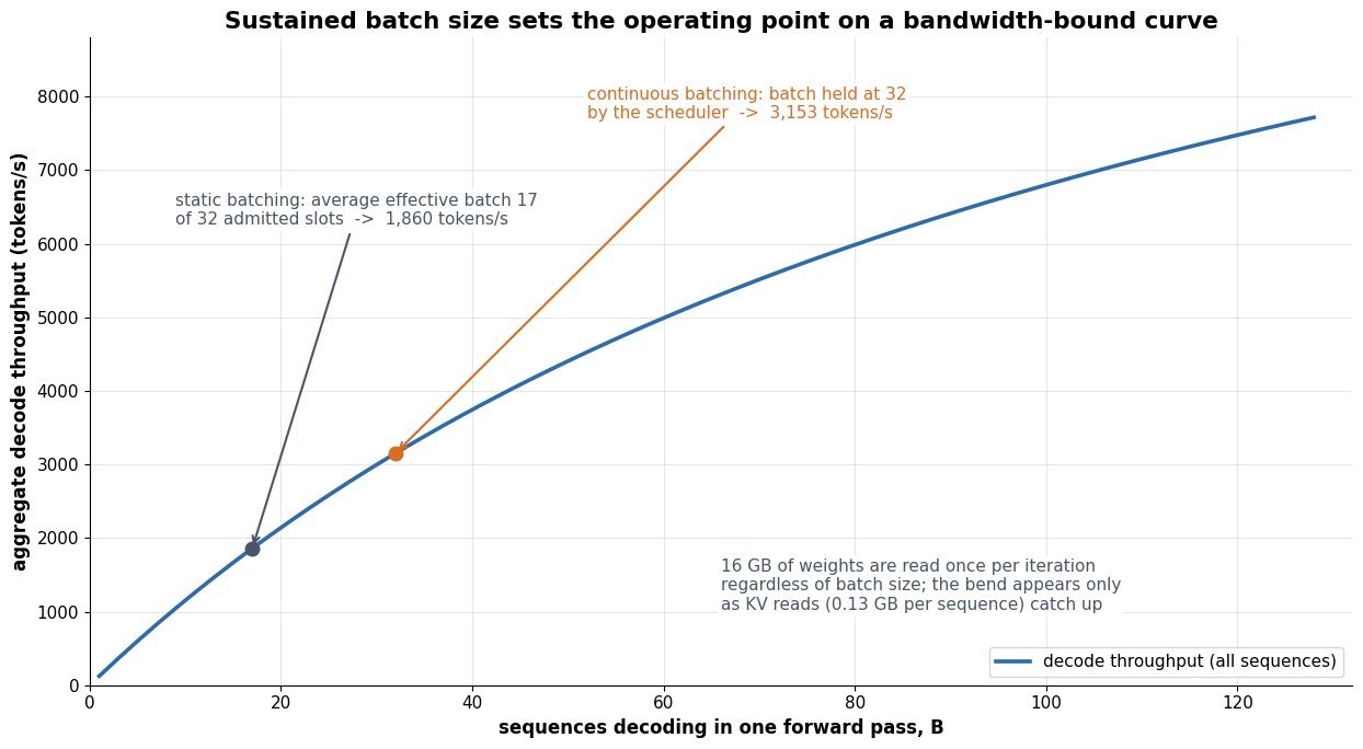
Figure 2: Decode throughput against sustained batch size for an 8B fp16 model with 1K-token contexts on a 2 TB/s GPU. The curve is bandwidth-bound everywhere in this range, so throughput rises almost linearly at small and bends only as KV reads start to rival the 16 GB weight read. Continuous batching does not move the curve; it moves the operating point, from the average effective batch a draining static group achieves to the memory-limited maximum.
Mathematical Formulation:


Where:
 is the fraction of batch slot-iterations that produce a token under static batching, with
  the output length of request
  and
and  ; it is exactly 1 only when all lengths are equal.
 is KV bytes per token, where
  is layers,
  key/value heads (small under GQA), head dimension,
  bytes per element, and the leading 2 counts K and V.
 is the parameter count, so
  bytes is the fp16 weight read paid once per iteration regardless of , and
  is achievable HBM bandwidth.
 is the mean context length in the running batch and the number of sequences decoding in one forward pass.
 is aggregate decode throughput in tokens per second; it is concave in because the KV term grows with while the weight term does not.
 is HBM left after weights and activations, so is the admission ceiling the scheduler targets; the formula assumes stays bounded, which it does not for sequences still growing.
 is the fraction of batch slot-iterations that produce a token under static batching, with
  the output length of request
  and
and  ; it is exactly 1 only when all lengths are equal.
 is KV bytes per token, where
  is layers,
  key/value heads (small under GQA),
  head dimension,
  bytes per element, and the leading 2 counts K and V.
 is the parameter count, so
  is achievable HBM bandwidth.
 is the mean context length in the running batch and
  is aggregate decode throughput in tokens per second; it is concave in
  is HBM left after weights and activations, so
 Throughput At Two Operating Points (8B fp16, 1K context, 2 TB/s):


The byte totals are the 16 GB weight read plus  GB of KV, divided by 2000 GB/s. Nearly doubling the sustained batch costs only 11% more time per step and yields 1.7x the tokens per second, which is the whole economic case for iteration-level scheduling: the extra sequences ride along in memory traffic that was already being paid.
| Property | Static (request-level) batching | Continuous (iteration-level) batching | Continuous + chunked prefill |
|---|---|---|---|
| Scheduling unit | One whole generation loop per group | One forward pass | One forward pass with a token budget split across prefill and decode |
| Wait for a new arrival | Until the longest sequence in the current group finishes | One iteration, if KV blocks are free | One iteration, and its prefill is spread over several |
| Wasted compute | Pad tokens plus idle slots, growing with length variance | Near zero: ragged attention, no padding | Near zero, with better SM occupancy on decode-only steps |
| KV memory model | Contiguous buffer reserved for max length per slot | Paged blocks allocated on demand, freed on retirement | Same paged blocks, filled incrementally during prefill |
| Inter-token latency | Stable within a group, terrible queueing before it | Spikes whenever a long prompt is admitted | Bounded by the chunk size, at slightly higher TTFT |
| Dominant failure mode | Throughput collapse under heavy-tailed output lengths | KV exhaustion causing preemption and recompute thrash | Chunk size mistuned, trading TTFT against throughput |
Leave a Reply