Interview for Machine Learning

Author: admin

ML0045 Multi-Layer Perceptron
What is a Multi-Layer Perceptron (MLP)? How does it overcome Perceptron limitations?
Answer
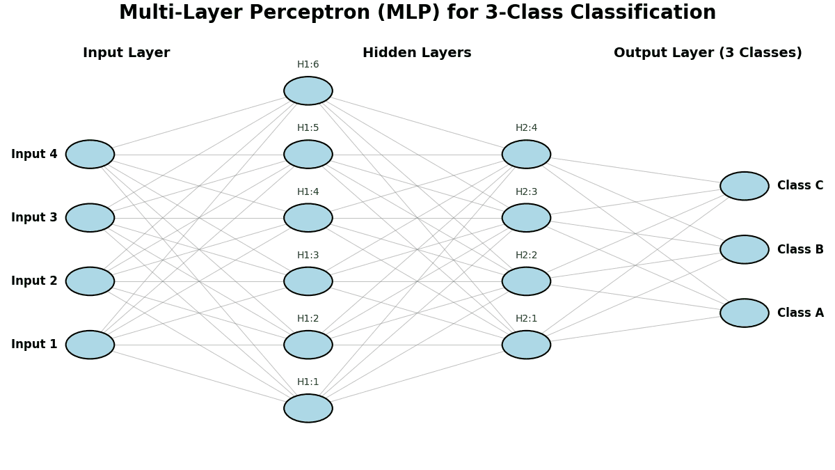
A Multi-Layer Perceptron (MLP) is a feedforward neural network with one or more hidden layers between the input and output layers. Hidden layers in MLP use non-linear activation functions (like ReLU, sigmoid, or tanh) to model complex relationships. MLP can be used for classification, regression, and function approximation. MLP is trained using backpropagation, which adjusts the weights to minimize errors.
Overcoming Limitations:
(1) Learn non-linear: Unlike a single-layer perceptron that can only solve linearly separable problems, an MLP can learn non-linear decision boundaries, handling problems such as the XOR problem.
(2) Universal Approximation: With enough neurons and layers, an MLP can approximate any continuous function, making it a powerful model for various applications.
The plot below illustrates an example of a Multi-Layer Perceptron (MLP) applied to a classification problem.
Login to view more content
May 26, 2025
ML0044 Perceptron
Describe the Perceptron and its limitations.
Answer
The perceptron is a simple linear classifier that computes a weighted sum of input features, adds a bias, and applies a step function to produce a binary decision. The perceptron works well only for data sets that are linearly separable, where a straight line (or hyperplane in higher dimensions) can separate the classes.
The perception output can be calculated by
$y = f(w^T x + b)$
Where:
$y$ is the predicted output (0 or 1)
$w$ is the weight vector
$x$ is the input vector
$b$ is the bias term
$f(\cdot)$ is the activation function (typically a step function)
Below shows a perceptron diagram.

Limitations for using perception:
(1) Linearly Separable Data Only: Cannot solve problems like XOR, which are not linearly separable.
(2) Single-Layer Only: Cannot model complex or non-linear patterns.
(3) No Probabilistic Output: Outputs only binary values, not confidence or probabilities.
Login to view more content
May 26, 2025
DL0015 Cold Start
What is a “cold start” problem in deep learning?
Answer
The cold start problem is the difficulty of making reliable predictions for new entities (such as users, items, or contexts) lacking historical data.
Many deep learning models, especially in recommendation systems, rely on abundant past data to learn meaningful patterns. When a new user or item is introduced, the model struggles because it doesn’t have enough information to produce accurate predictions.
Mitigation Strategies for the Cold Start Problem:
(1) Transfer Learning / Pretrained Models: Use embeddings or models pre-trained on similar tasks to provide a starting point.
(2) Hybrid Recommendation Models: Combine collaborative filtering (CF) and content-based methods.
(3) Active Learning / User Onboarding: Actively gather more data for new entities through user interactions.
Login to view more content
May 26, 2025
ML0043 Feature Scaling
Walk me through the rationale behind Feature Scaling in machine learning.
Answer
Feature scaling is a fundamental data preprocessing step that normalizes or standardizes the range of numerical features. It is essential for many machine learning algorithms to ensure that all features contribute equally to the model, leading to faster convergence, improved accuracy, and better overall model performance, especially for algorithms sensitive to the magnitude of feature values or those based on distance calculations.
Definition: Process of normalizing or standardizing input features so they’re on a similar scale.
Why Needed: Many ML models (e.g., SVM, KNN) are sensitive to feature magnitude. Prevents dominant features from overpowering others due to scale.
Common Methods:
Min-Max Scaling: Scales features to a range (usually [0, 1]).
$\mbox \quad X_{\text{normalized}} = \frac{X - X_{\text{min}}}{X_{\text{max}} - X_{\text{min}}}$
Where:
$X$ represents the original value of the feature.
$X_{\text{min}}$ represents the minimum value of the feature in the dataset.
$X_{\text{max}}$ represents the maximum value of the feature in the dataset.
Standardization (Z-score Normalization, centers data to mean 0, standard deviation to 1):
$\mbox \quad X_{\text{standardized}} = \frac{X - \mu}{\sigma}$
Where:
$X$ represents the original value of the feature.
$\mu$ represents the mean of the feature in the dataset.
$\sigma$ represents the standard deviation of the feature in the dataset.
Below shows an example plot for original, min-max scaled, and standardized data.
Login to view more content
May 25, 2025
ML0042 Early Stopping
What is Early Stopping? How is it implemented?
Answer
Early Stopping is a regularization technique used to halt training when a model’s performance on a validation set stops improving, thus avoiding overfitting. It monitors metrics like validation loss or validation accuracy and stops after a defined number of stagnant epochs (patience). This ensures efficient training and better generalization.
Implementation:
Split data into training and validation sets.
After each epoch, evaluate on the validation set.
If performance improves, save the model and reset the patience counter.
If no improvement, counter add one; if the counter reaches the patience epochs, stop training.
Restore best weights after stopping, load the model weights from the epoch that yielded the best validation performance.
Below is one example loss plot when using early stop.
Login to view more content
May 25, 2025
ML0041 Concept of NN
Please explain the concept of a Neural Network.
Answer
A neural network (NN) is a machine learning model composed of layers of interconnected neurons. It learns patterns in data by adjusting weights through training, enabling it to perform tasks like classification, regression, and more.
(1) Inspired by Biology: Neural networks are computer systems modeled after the human brain’s network of neurons.
(2) Layered Structure: Neural networks consist of an input layer, one or more hidden layers, and an output layer.
(3) Neurons and Activation: Each neuron performs a weighted sum of its inputs, adds a bias, and applies an activation function to produce an output. Weights and Biases are learnable parameters adjusted during training. Activation Functions can introduce non-linearity (e.g., ReLU, Sigmoid).
(4) Learning Process: Neural networks learn by adjusting the weights and biases through training algorithms such as backpropagation, minimizing errors between predictions and actual results.
(5) Versatility in Applications: Neural networks can identify complex patterns, making them suitable for tasks like image recognition, natural language processing, and data classification.
Below shows an example of an NN.
Login to view more content
May 24, 2025
DL0014 Mixed Precision Training
Can you explain the primary benefits of using mixed precision training in deep learning?
Answer
Mixed precision training accelerates deep learning by using both FP32 and FP16 operations, which reduces memory and computational requirements while maintaining model accuracy, resulting in faster and more efficient training.
(1) Faster Training: Uses lower-precision (e.g., FP16) operations on supported hardware (like GPUs/TPUs), which are faster than FP32.
(2) Reduced Memory Usage: Lower-bit representations decrease memory footprint, allowing larger batch sizes or models.
(3) Higher Throughput: More computations per second due to reduced precision, which can speed up training time.
(4) Supports Large Models: Enables training of models that wouldn’t fit in memory with full precision.
(5) Maintains Accuracy: With proper scaling (e.g., loss scaling), training stability and final model accuracy can typically be preserved.
Login to view more content
May 22, 2025
DL0013 Instance Normalization
Can you explain what Instance Normalization is in the context of deep learning?
Answer
Instance Normalization (IN) normalizes each individual data sample (often per channel) by subtracting its own mean and dividing by its variance, then applying a scale and shift. This makes it ideal for applications where per-instance adjustment is needed, such as artistic style transfer, ensuring that the normalization is not affected by the mini-batch composition.
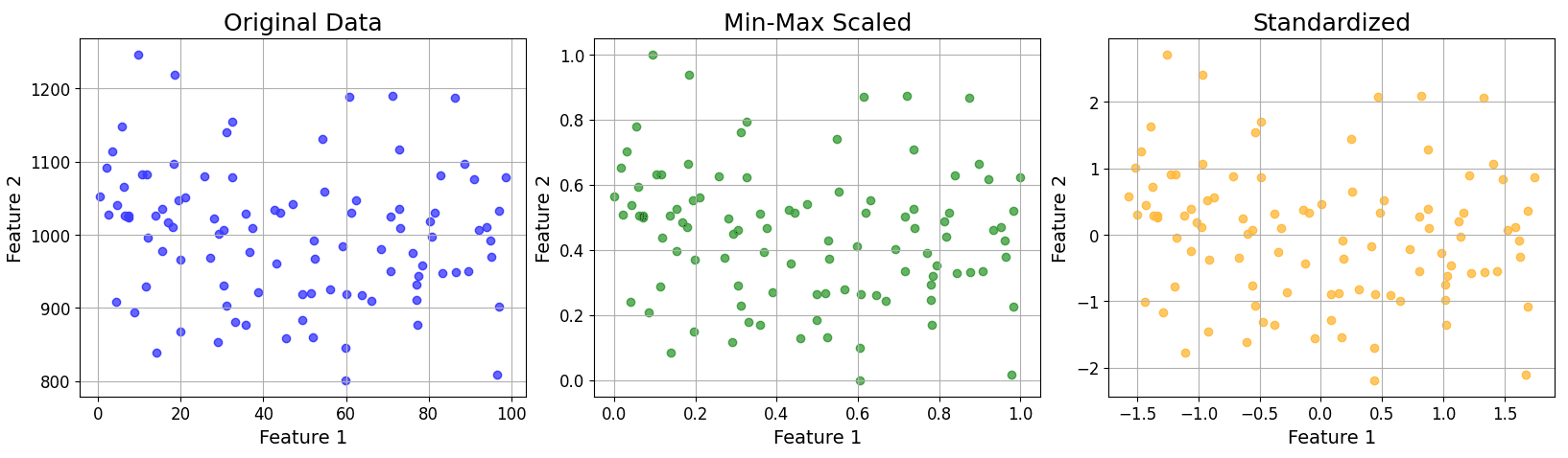
Here are the equations for calculating Instance Normalization output $y_{nchw}$ for input $x_{nchw}$ :
$\mu_{nc} = \frac{1}{HW} \sum_{h=1}^{H} \sum_{w=1}^{W} x_{nchw}$
$\sigma_{nc}^2 = \frac{1}{HW} \sum_{h=1}^{H} \sum_{w=1}^{W} (x_{nchw} - \mu_{nc})^2$
$\hat{x}_{nchw}=\frac{{x}_{nchw} - \mu_{nc}}{\sqrt{\sigma_{nc}^2 + \epsilon}}$
$y_{nchw} = \gamma_c \hat{x}_{nchw} + \beta_c$
Where:
$x_{nchw}$ is the input feature at batch $n$ , channel $c$ , height $h$ , and width $w$ .
$H$ is the height of the feature map (number of rows per channel).
$W$ is the width of the feature map (number of columns per channel).
$\mu_{nc}$ is the mean of all spatial values in channel $c$ of instance $n$ .
$\sigma_{nc}^2$ is the variance of spatial values in channel $c$ of instance $n$ .
$\hat{x}_{nchw}$ is the normalized value after subtracting the mean and dividing by the standard deviation.
$\epsilon$ is a small constant added to the denominator to prevent division by zero and improve numerical stability.
$y_{nchw}$ is the final output after applying normalization and scaling.
$\gamma_c$ is a learnable scale parameter for channel $c$ .
$\beta_c$ is a learnable shift parameter for channel $c$ .
Login to view more content
May 22, 2025
ML0040 Bias and Variance
Can you explain the bias-variance tradeoff?
Answer
Bias:
Error due to overly simplified assumptions in the model.
High bias may lead to underfitting, where the model misses key patterns in the data.
Variance:
Error due to high sensitivity to variations in the training data.
High variance may result in overfitting, where the model captures noise and underlying patterns.
Bias-Variance Tradeoff:
Increasing model complexity typically decreases bias but increases variance, while a simpler model increases bias but decreases variance.
The goal is to balance both to minimize the total error on unseen data.
The bias-variance tradeoff illustrates that there’s a delicate balance to strike when building a machine learning model. A simpler model tends to have high bias and low variance, underfitting the data. A more complex model tends to have low bias and high variance, overfitting the data. The goal is to find the right level of model complexity to minimize the total prediction error, which is the sum of squared bias, variance, and irreducible error.
The example below shows scenarios of high bias (underfitting), high variance (overfitting), and a good balance.
Login to view more content
May 21, 2025
ML0039 Distributed Training
What are the two main distributed training approaches for machine learning?
Answer
The two main distributed training approaches for machine learning are Data Parallelism and Model Parallelism.
Data Parallelism: In this approach, the training dataset is divided and distributed among multiple computing devices, with each device holding a complete copy of the machine learning model. Each device then trains its model on its assigned subset of the data in parallel. After each training step, the updates (gradients or new parameters) from all devices are aggregated and synchronized to maintain a consistent model across the system. This method is highly effective for scaling training when the dataset is large and the model can fit within a single device’s memory.
Model Parallelism: This approach is used when the machine learning model itself is too large to fit into the memory of a single computing device. In model parallelism, different parts of the model (e.g., specific layers of a neural network) are distributed across multiple devices. Data typically flows sequentially through these distributed model parts. This necessitates more complex communication between devices as intermediate computations and activations must be passed along. Model parallelism is crucial for training extremely large models that would otherwise be computationally intractable on a single machine.
Login to view more content
May 21, 2025