Author: admin

  • ML0043 Feature Scaling

    Walk me through the rationale behind Feature Scaling in machine learning.

    Answer

    Feature scaling is a fundamental data preprocessing step that normalizes or standardizes the range of numerical features, so all features contribute equally to the model. It leads to faster convergence, improved accuracy, and better overall performance, especially for algorithms sensitive to feature magnitudes or based on distance calculations (e.g., SVM, KNN), where an unscaled large-range feature would overpower the others.

    (1) Definition: Normalize or standardize input features so they sit on a similar scale.
    (2) Why Needed: Many ML models are sensitive to feature magnitude; scaling prevents dominant features from overwhelming the rest purely because of their units.
    (3) Two Common Methods: Min-max scaling maps features to a fixed range (usually [0, 1]); standardization (z-score) centers features to mean 0 and standard deviation 1.

    Three scatter panels showing the same dataset as original features, min-max scaled to the unit square, and standardized to zero mean unit variance

    Figure 1: The same 100 samples under the two scalings: the original features live on incompatible scales (Feature 1 in [0, 100], Feature 2 around 1000); min-max compresses both axes into [0, 1]; standardization centers the cloud at the origin with unit spread. The shape of the point cloud is preserved: only the units change.

    Mathematical Formulation:
    X_{\text{normalized}} = \frac{X - X_{\text{min}}}{X_{\text{max}} - X_{\text{min}}}
    X_{\text{standardized}} = \frac{X - \mu}{\sigma}

    Where:

    • X is the original feature value.
    • X_{\text{min}} and X_{\text{max}} are the feature’s minimum and maximum in the training data.
    • \mu and \sigma are the feature’s mean and standard deviation in the training data.

    Login to view more content
  • ML0042 Early Stopping

    What is Early Stopping? How is it implemented?

    Answer

    Early stopping is a regularization technique that halts training when the model’s performance on a validation set stops improving, thus avoiding overfitting. It monitors a metric such as validation loss or validation accuracy and stops after a defined number of stagnant epochs (the patience). This ensures efficient training and better generalization.

    (1) Split Data: Reserve a validation set separate from the training set.
    (2) Evaluate Each Epoch: After every training epoch, measure performance on the validation set.
    (3) Track Improvement: If performance improves, save the model and reset the patience counter; if not, increment the counter; when it reaches the patience, stop training.
    (4) Restore Best Weights: After stopping, reload the weights from the epoch that yielded the best validation performance, not the final epoch.

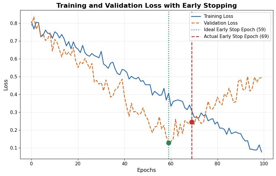
    Training loss keeps decreasing while validation loss bottoms out at epoch 60 and rises again, with the actual stop at epoch 70 under patience 10

    Figure 1: Early stopping in action: training loss falls monotonically, but validation loss bottoms out at epoch 60 (ideal stop) and then rises as the model overfits. With patience 10, training actually halts at epoch 70 and the weights from epoch 60 are restored.

    Mathematical Formulation:
    t^* = \arg\min_{t} \; \mathcal{L}_{\text{val}}\big(\theta_t\big)
    \text{stop at } t^* + p \text{ if no epoch in } (t^*,\, t^* + p] \text{ beats } \mathcal{L}_{\text{val}}(\theta_{t^*})

    Where:

    • \theta_t are the model weights after epoch t; \mathcal{L}_{\text{val}} is the validation loss.
    • t^* is the epoch with the best validation loss, the checkpoint whose weights are restored at the end.
    • p is the patience: how many consecutive non-improving epochs are tolerated before stopping.

    Login to view more content
  • ML0041 Concept of NN

    Please explain the concept of a Neural Network.

    Answer

    A neural network (NN) is a machine learning model composed of layers of interconnected neurons. It learns patterns in data by adjusting weights through training, enabling tasks like classification, regression, and more. Neural networks are inspired by biology (they are computer systems modeled after the human brain’s network of neurons), and they excel at identifying complex, non-linear patterns, which makes them suitable for image recognition, natural language processing, and data classification.

    (1) Layered Structure: A neural network consists of an input layer, one or more hidden layers, and an output layer; data flows from input to output through the hidden layers.
    (2) Neurons And Activation: Each neuron computes a weighted sum of its inputs, adds a bias, and applies an activation function. Weights and biases are learnable parameters adjusted during training, and activation functions (e.g., ReLU, sigmoid) introduce the non-linearity that lets the network model complex relationships.
    (3) Learning Process: The network learns by adjusting weights and biases through training algorithms such as backpropagation, minimizing the error between its predictions and the actual results.

    Feedforward neural network with a three node input layer, a five node hidden layer, and a two node output layer, fully connected

    Figure 1: A feedforward neural network: every neuron in one layer connects to every neuron in the next. Each connection carries a learned weight; each hidden and output neuron adds a bias and applies an activation function.

    Mathematical Formulation:
    a_j = f\Big(\sum_{i} w_{ji}\, x_i + b_j\Big)

    Where:

    • x_i are the inputs to the neuron (raw features for the input layer, previous-layer activations otherwise).
    • w_{ji} is the weight on the connection from input i to neuron j; b_j is the neuron’s bias; both are learned during training.
    • f(\cdot) is the activation function (ReLU, sigmoid, tanh, …); a_j is the neuron’s output passed to the next layer.

    Login to view more content
  • DL0014 Mixed Precision Training

    Can you explain the primary benefits of using mixed precision training in deep learning?

    Answer

    Mixed precision training runs the compute-heavy parts of a model in FP16 while keeping an FP32 master copy of the weights, so training gets the speed and memory of half precision without sacrificing final accuracy. Modern GPU/TPU tensor cores execute FP16 matrix math several times faster than FP32, and halving activation memory lets you train larger models or use larger batches on the same hardware.

    (1) Faster Training: FP16 tensor-core matmuls deliver up to an order of magnitude more throughput than FP32 on supported hardware (e.g., ~312 vs ~19.5 TFLOPS on an A100).
    (2) Reduced Memory Usage: FP16 activations and working weight copies occupy half the bytes, freeing room for larger batch sizes or deeper models (master weights and optimizer states stay FP32, so total training memory falls by less than half).
    (3) Maintained Accuracy: FP32 master weights plus loss scaling keep small gradient values representable, so final model quality matches full-precision training.

    Bit layout comparison of FP32 with 8 exponent and 23 mantissa bits versus FP16 with 5 exponent and 10 mantissa bits, showing the reduced dynamic range of FP16.

    Figure 1: FP16 trades exponent range and mantissa precision for half the storage: gradients below 6.1 \times 10^{-5} would underflow to zero without loss scaling.

    The Training Loop: Weights are stored in FP32 as the master copy. Each step casts them to FP16 for the forward and backward passes, multiplies the loss by a scale factor S so that FP16 gradients stay in range, then divides the gradients by S and applies the optimizer update to the FP32 master weights.

    Mixed precision training loop diagram showing FP32 master weights cast to FP16 for forward and backward passes with loss scaling, then unscaled gradients updating the FP32 master copy.

    Figure 2: FP16 does the heavy math while the FP32 master copy absorbs tiny updates; loss scaling S shifts gradients into FP16’s representable range.

    Measured Benefits: On tensor-core hardware the speedup is substantial, and the halved activation memory (the dominant term at large batch sizes) directly translates into larger feasible models or batches.

    Bar charts comparing FP32 versus mixed precision on tensor-core throughput and per-parameter memory footprint.

    Figure 3: Roughly 16x tensor-core throughput and half the activation memory are the headline wins; with Adam states kept in FP32, per-parameter training memory drops only modestly.

    Mathematical Formulation:
    \mathcal{L}' = S \cdot \mathcal{L}
    g_{fp32} = \frac{1}{S}\,\nabla_{\theta}\mathcal{L}'
    \theta \leftarrow \theta - \eta\, g_{fp32}

    Where:

    • S is the loss-scale factor (e.g., 2^{15}, or dynamically adjusted); \mathcal{L}' is the scaled loss used for backprop in FP16.
    • \nabla_{\theta}\mathcal{L}' are the scaled FP16 gradients; dividing by S restores the true gradient g_{fp32}.
    • \theta is the FP32 master weight set and \eta the learning rate; updates always land on the master copy.

    Costs to Manage: FP16’s narrow range causes gradient underflow and occasional activation overflow, requiring loss scaling and careful debugging of NaN/Inf values; efficiency also depends on hardware with fast FP16 paths.


    Login to view more content
  • DL0013 Instance Normalization

    Can you explain what Instance Normalization is in the context of deep learning?

    Answer

    Instance Normalization (IN) normalizes each individual sample and each channel independently: for every (instance, channel) pair it subtracts the mean and divides by the standard deviation computed over that feature map’s spatial dimensions only. Because statistics never cross instance boundaries, IN is unaffected by mini-batch composition and works with batch size 1. This per-instance normalization removes sample-specific contrast and style, which is why IN became the standard in style transfer and image-generation models.

    (1) Per-Instance, Per-Channel Statistics: Mean and variance are computed over the H \times W spatial positions of each channel of each sample separately, so no information leaks across the batch.
    (2) Batch-Size Independent: Statistics do not depend on other samples, so IN behaves identically at training and test time and remains stable with small batches.
    (3) Removes Instance-Specific Style: Normalizing each map’s contrast discards style-like appearance information while preserving content structure, which suits style transfer, GANs, and domain adaptation.

    Side-by-side diagram of batch normalization sharing per-channel statistics across all instances versus instance normalization computing statistics within each instance-channel feature map.

    Figure 1: BN pools statistics per channel across the whole batch (red dashed groups), while IN normalizes each (instance, channel) map alone (orange dashed boxes): the source of IN’s batch independence.

    Mathematical Formulation:
    \mu_{nc} = \frac{1}{HW} \sum_{h=1}^{H} \sum_{w=1}^{W} x_{nchw}
    \sigma_{nc}^2 = \frac{1}{HW} \sum_{h=1}^{H} \sum_{w=1}^{W} (x_{nchw} - \mu_{nc})^2
    \hat{x}_{nchw} = \frac{x_{nchw} - \mu_{nc}}{\sqrt{\sigma_{nc}^2 + \epsilon}}
    y_{nchw} = \gamma_c\,\hat{x}_{nchw} + \beta_c

    Where:

    • x_{nchw} is the input activation at batch index n, channel c, spatial position (h, w).
    • \mu_{nc} and \sigma_{nc}^2 are the mean and variance over the H \times W spatial extent of instance n, channel c.
    • \hat{x}_{nchw} is the normalized activation; \epsilon is a small constant for numerical stability.
    • \gamma_c and \beta_c are learnable per-channel scale and shift parameters; y_{nchw} is the output.

    Contrast with Batch Normalization: BN computes per-channel statistics over the entire mini-batch (N \times H \times W), which couples a sample’s output to its batchmates and forces a switch to running averages at inference. IN’s per-sample statistics are identical in both phases, and discarding per-instance contrast is precisely what removes style from content images.

    FeatureInstance Normalization (IN)Batch Normalization (BN)
    Scope of statsPer instance, per channel (over H \times W)Per channel (over N \times H \times W)
    Batch sizeIndependent; works with batch = 1Dependent; needs stable batch stats
    Primary useStyle transfer, GANs, domain adaptationImage classification, general CNNs
    EffectRemoves instance-specific style/contrastStabilizes training, speeds convergence
    InferenceSame per-sample stats at test timeUses running stats from training

    Bottom line: IN removes per-instance contrast (style); BN aligns feature scales across the batch. IN trades BN’s cross-sample regularization for batch independence and style removal.


    Login to view more content
  • ML0040 Bias and Variance

    Can you explain the bias-variance tradeoff?

    Answer

    The bias-variance tradeoff decomposes a model’s expected prediction error into three parts: squared bias, variance, and irreducible noise. Bias is the error from overly simplified assumptions: a high-bias model misses the real pattern and underfits. Variance is the error from sensitivity to the particular training sample: a high-variance model wiggles to fit noise and overfits. The tradeoff arises because increasing model complexity typically decreases bias but increases variance, while simplifying does the reverse: total error as a function of complexity is U-shaped, and the goal is the sweet spot that minimizes the sum. Practically, high bias shows as large training error; high variance shows as a large gap between training and validation error, and each has its own remedies (more capacity/features for bias; more data, regularization, or simpler models for variance).

    (1) Bias: Error from wrong assumptions: underfitting, poor fit on both train and test data.
    (2) Variance: Error from sample sensitivity: overfitting, big train/test gap.
    (3) Tradeoff: Complexity trades one for the other; total error = \text{Bias}^2 + \text{Variance} + \sigma^2 is U-shaped: minimize the sum.

    Bias squared decreasing, variance increasing, and U-shaped total error versus model complexity with the optimum marked

    Figure 1: The classic tradeoff curve: bias² falls and variance rises as complexity grows; total error is their U-shaped sum, and the best model sits at the minimum, not at maximum complexity.

    Mathematical Formulation:
    \mathbb{E}\big[(y - \hat{f}(x))^2\big] = \underbrace{\big(\mathbb{E}[\hat{f}(x)] - f(x)\big)^2}_{\text{Bias}^2} + \underbrace{\mathbb{E}\big[(\hat{f}(x) - \mathbb{E}[\hat{f}(x)])^2\big]}_{\text{Variance}} + \underbrace{\sigma^2}_{\text{noise}}

    Where:

    • f(x) is the true relationship and \hat{f}(x) the model’s prediction; expectations are over training sets.
    • \text{Bias}^2 measures how far the average model is from the truth; \text{Variance} how much predictions scatter around that average.
    • \sigma^2 is the irreducible error: noise in the data itself that no model can eliminate.
    Three panels showing underfitting with high bias, a good balance fit, and overfitting with high variance

    Figure 2: The tradeoff on real-shaped data: the high-bias model is too rigid to follow the curve (both errors high); the high-variance model chases every noisy point (train error low, test error high); the balanced model tracks the true function and minimizes test error.


    Login to view more content
  • ML0039 Distributed Training

    What are the two main distributed training approaches for machine learning?

    Answer

    The two main distributed training approaches are data parallelism and model parallelism, and they answer different bottlenecks. In data parallelism, the dataset is split across many devices, each holding a complete copy of the model; every device computes gradients on its own mini-batch, and after each step the gradients are aggregated and synchronized so all copies stay identical. It scales training when the data is large but the model still fits in one device’s memory. In model parallelism, the model itself is too large for one device, so different parts of the model (e.g., different layers) are placed on different devices, and data flows through them in sequence, with activations passed between devices. It is the enabling technique for today’s very large models, at the cost of more complex communication. Modern large-scale training often combines both (plus pipeline and tensor parallelism) in hybrid strategies.

    (1) Data Parallelism: Full model copy per device, different data shards, gradients synchronized after each step: scales with data.
    (2) Model Parallelism: The model is split across devices, data flows sequentially through the parts: scales with model size.
    (3) Trade-off: Data parallel communicates gradients per step; model parallel communicates activations between stages.

    Data parallelism with model replicas on three GPUs training on data shards versus model parallelism with layers split across three GPUs

    Figure 1: The two approaches: data parallelism (left) replicates the whole model on every device and splits the data, synchronizing gradients after each step; model parallelism (right) splits the model itself across devices and passes activations down the chain.

    Mathematical Formulation:
    g = \frac{1}{D} \sum_{d=1}^{D} g_d
    g_d = \nabla_\theta \mathcal{L}_d(\theta) \quad \text{(data-parallel gradient sync)}
    h^{(d+1)} = f^{(d+1)}\big(h^{(d)};\, \theta^{(d+1)}\big)
    \theta^{(d+1)} \text{ lives on device } d+1 \text{ (model parallel)}

    Where:

    • D is the number of devices; g_d the gradient computed by device d on its data shard; g the synchronized average applied to every replica.
    • h^{(d)} is the activation handed from device d to device d+1; \theta^{(d)} the slice of parameters owned by device d.

    Login to view more content
  • ML0038 Validation and Test

    What are the key purposes of using both a validation and a test set when building machine learning models?

    Answer

    The validation set and the test set play two different roles that must not be merged: validation guides every development decision, the test set is touched exactly once for the final unbiased verdict. During development you use the validation set to tune hyperparameters (learning rate, architecture, regularization), select among candidate models, and monitor overfitting (e.g., for early stopping): it is the “unseen” data you are allowed to peek at repeatedly. But because those repeated peeks gradually fit your decisions to the validation set, its score becomes optimistically biased. The test set therefore stays locked away until the model and all its settings are frozen: evaluating on it once simulates real-world performance on genuinely unseen data and guarantees no information from it leaked into any modeling choice. Using the validation set as the test set destroys that guarantee; with very scarce data, rigorous cross-validation during development is the acceptable compromise.

    (1) Validation Set: Tunes hyperparameters, selects models, watches for overfitting: the decision-making dataset.
    (2) Test Set: One-shot final evaluation of the frozen model: the unbiased estimate of real-world performance.
    (3) Separation Why: Repeated validation peeking biases its score; only an untouched set can certify generalization.

    Workflow of training set fitting candidates, validation set selecting the best, and test set used once for the final score

    Figure 1: The role of each split: the training set fits many candidates; the validation set is queried repeatedly to tune and pick the winner (feedback loop); the test set is used exactly once, after everything is frozen; no arrow leads back from it.

    Mathematical Formulation:
    \hat{\lambda} = \arg\min_{\lambda} \; \mathcal{L}_{\text{val}}\big(\hat{\theta}(\lambda)\big)
    \hat{\theta}(\lambda) = \arg\min_{\theta} \; \mathcal{L}_{\text{train}}(\theta; \lambda)
    \text{Final estimate:} \quad \mathcal{L}_{\text{test}}\big(\hat{\theta}(\hat{\lambda})\big) \quad \text{(computed once, model frozen)}

    Where:

    • \theta are model parameters fitted on the training set; \lambda the hyperparameters chosen on the validation set.
    • \mathcal{L}_{\text{val}} is optimized indirectly through many modeling decisions, so it underestimates true error; \mathcal{L}_{\text{test}} enters no optimization and stays unbiased.

    Login to view more content
  • ML0037 Bias in NN

    Why is bias used in neural networks?

    Answer

    The bias term in a neuron (z = Wx + b) is the learnable offset that shifts the activation function’s threshold. Without it, every neuron’s pre-activation would be a strictly linear (origin-passing) function of its inputs: a neuron could only fire proportionally to its input, and every decision boundary or fitted function would be forced through the origin. The bias removes that constraint: it lets a neuron activate even when its weighted input sums to zero, and lets decision boundaries sit anywhere in input space, not just through the origin. This adds crucial flexibility for approximating real-world functions, compensates for systematic offsets in the data, and plays a role loosely analogous to the firing threshold of a biological neuron: the bias sets how much input stimulation is needed before the neuron becomes active. In short, the bias is to a neuron what the intercept is to linear regression: a small parameter with an outsized effect on representational power.

    (1) Shifts the Threshold: The bias moves the activation curve left/right, so a neuron can fire (or stay off) at any input level.
    (2) Escapes the Origin: Without bias, boundaries and fitted functions are forced through (0,0); with it they can sit anywhere.
    (3) Flexibility: One extra learnable parameter per neuron that absorbs systematic offsets and improves approximation.

    Data whose trend misses the origin, fitted poorly by a no-bias line forced through the origin and well by a line with bias

    Figure 1: Why bias matters in one picture: the data’s trend clearly does not pass through the origin. The no-bias model (orange) is constrained through (0,0) and misfits everywhere; the model with a bias term (blue) shifts the line up and fits the trend.

    Mathematical Formulation:
    z = \sum_{i} w_i x_i + b = Wx + b
    a = f(z)
    z > 0 \Leftrightarrow \sum_i w_i x_i > -b

    Where:

    • x_i are the inputs, w_i the weights, b the bias, z the pre-activation, a the output.
    • -b acts as the effective threshold: the third line says the unit crosses its threshold exactly when the weighted input exceeds -b. With b > 0 the neuron activates more easily (even at zero input); with a negative bias it requires stronger input to fire.

    Login to view more content
  • ML0036 Confusion Matrix

    In which scenarios is a Confusion Matrix most useful for evaluating machine learning models, and why?

    Answer

    A confusion matrix tabulates a classifier’s predictions against the true labels (in the binary case the four counts TP, FP, FN, and TN), so it exposes not just how many errors a model makes but which kinds. It earns its place whenever a single scalar metric would hide something important. On imbalanced datasets it reveals whether the minority class is actually being found: a model scoring 95% accuracy by mostly ignoring a 5% class is exposed instantly by its minority row. When error types have different costs (medical screening, fraud detection), the FP and FN cells let you weigh false alarms against misses explicitly. In multi-class problems, off-diagonal clusters show which specific classes the model confuses, guiding targeted fixes. It is also the right tool for model comparison beyond one metric, and for stakeholder communication: “we caught X% of positives while mis-flagging Y% of negatives” makes trade-offs concrete for non-technical audiences.

    (1) Imbalanced Data: Minority-class performance is visible row by row; accuracy alone would hide it.
    (2) Asymmetric Costs: FP and FN are separated, so false-alarm vs miss trade-offs can be tuned deliberately.
    (3) Diagnosis: Multi-class off-diagonals show exactly which classes get confused; four-quadrant views communicate clearly to stakeholders.

    Binary confusion matrix heatmap with counts on the diagonal and small off-diagonal errors

    Figure 1: A binary confusion matrix: the strong diagonal (87 and 89 correct) shows a healthy classifier, while the small off-diagonal cells (10 false alarms, 14 misses) quantify the two error types separately, information accuracy alone cannot give.

    Mathematical Formulation:
    M_{ij} = \sum_{k=1}^{N} \mathbb{1}\big(y_k = i,\; \hat{y}_k = j\big)
    \text{precision} = \frac{TP}{TP + FP}
    \text{recall} = \frac{TP}{TP + FN}
    \text{accuracy} = \frac{TP + TN}{N}

    Where:

    • M_{ij} counts samples whose true class is i and predicted class is j; \mathbb{1}(\cdot) is the indicator function.
    • TP, FP, FN, TN are the four binary cells: correct positives, false alarms, misses, and correct negatives.
    • Every standard classification metric is an arithmetic combination of the cells: the matrix is the source, the metrics are views of it.

    Login to view more content