Author: admin

  • DL0020 CNN Parameter Sharing

    How do Convolutional Neural Networks achieve parameter sharing? Why is it beneficial?

    Answer

    CNNs share parameters by applying the same convolutional filter at every spatial location: a small kernel of learnable weights slides across the input, and its weights are reused to compute each output activation. This weight reuse means the network learns location-independent features with far fewer parameters than a fully connected layer, which improves generalization and compute efficiency.

    How Sharing Works:

    (1) Convolutional Filter: A small matrix of learnable weights (e.g., 3 \times 3) is defined per channel pair.
    (2) Sliding Window: The filter moves across the whole input feature map, position by position.
    (3) Weight Reuse: The identical weights are used at every position, so one filter detects its feature anywhere in the image.
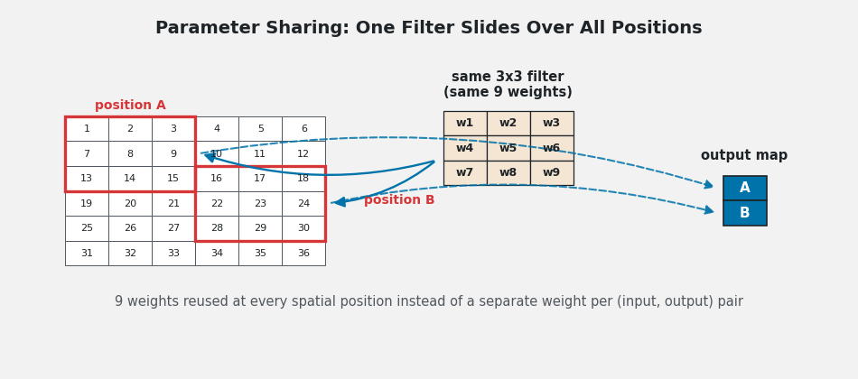
    Diagram of one shared 3x3 filter with the same nine weights applied at two different positions of an input grid producing two output activations.

    Figure 1: The same 9 weights produce activations at position A and position B. No new parameters are added as the input grows.

    Why It Is Beneficial:

    (1) Reduced Parameters: A filter has k \times k \times C_{in} weights regardless of input resolution, versus one weight per (input, output) pair in an FC layer.
    (2) Translation Equivariance: A feature detected at one location is detected at any location; shifting the input shifts the output correspondingly.
    (3) Improved Generalization: Fewer parameters means less overfitting, especially on limited data.
    (4) Computational Efficiency: Fewer parameters mean fewer multiply-accumulates in both forward and backward passes, enabling deployment on resource-limited devices.
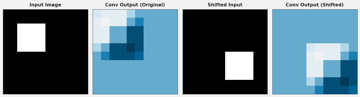
    Four panels showing an input image with a square, its convolution output, a shifted input, and the identically shifted convolution output demonstrating translation equivariance.

    Figure 2: Translation equivariance in action: shifting the input shifts the convolution output by the same amount, because the same shared filter processes every position.

    How Big Is the Saving? Sharing decouples the parameter count from the input resolution: growing the image grows the compute, not the weights. The contrast with a fully connected layer on the same input is dramatic.

    Log-scale bar chart comparing about 307 thousand parameters for a fully connected layer on a 32x32x3 input versus about 1.8 thousand for a shared 3x3 convolution.

    Figure 3: Flattening a 32 \times 32 \times 3 image into 100 FC units needs ~307k parameters; a shared 3 \times 3 convolution with 64 filters needs ~1.8k, roughly 170x fewer.

    Mathematical Formulation:
    y_{ijc} = \sum_{a=1}^{k}\sum_{b=1}^{k}\sum_{d=1}^{C_{in}} w_{abdc}\, x_{i+a,\, j+b,\, d} + b_c
    P_{conv} = k^2 \cdot C_{in} \cdot C_{out} + C_{out}

    Where:

    • y_{ijc} is the output activation at spatial position (i, j) of channel c; the same w is used for every (i, j): that reuse is parameter sharing.
    • w_{abdc} is the filter weight at kernel offset (a, b) connecting input channel d to output channel c; b_c is the per-output-channel bias.
    • P_{conv} is the layer’s parameter count, independent of the input’s spatial size H \times W.

    Login to view more content
  • DL0019 Go Deep

    How does increasing network depth impact the learning process?

    Answer

    Increasing network depth enhances feature learning and model capacity, but brings training instability, higher computational cost, and design complexity. Deeper stacks learn hierarchical representations (edges become textures, shapes, then objects) and can express certain complex functions far more efficiently than shallow networks, yet without modern techniques like residual connections and normalization, very deep networks are difficult or impossible to train.

    Benefits of Depth:

    (1) Improved Feature Hierarchy: Each layer composes the previous layer’s features, building increasingly abstract, high-level representations.
    (2) Increased Model Capacity: More layers let the network model more complex functions and patterns.
    (3) Exponential Efficiency for Complex Functions: Deep networks can represent some functions with vastly fewer units. For example, the n-input parity function needs roughly 2^{n-1} neurons in a single hidden layer but only about n small layers in a deep network.

    Challenges of Depth:

    (1) Vanishing/Exploding Gradients: Gradients shrink or grow multiplicatively through layers; without skip connections a 100-layer network may fail to train because gradients vanish before reaching early layers.
    (2) Increased Computational Cost: Deeper networks need significantly more compute and training time.
    (3) Higher Data Requirements: More parameters mean more overfitting risk unless the dataset grows correspondingly.

    Curve comparison showing a deep network tracking a complex high-frequency target function closely while a shallow network with a single hidden layer smooths over fine structure.

    Figure 1: A 6-layer network tracks the target’s high-frequency detail that a single-hidden-layer network smooths over. Depth buys compositional expressiveness.

    Where Depth Hurts Training: Each layer multiplies gradients by its Jacobian, so gradient magnitude behaves like a product of many factors; it collapses exponentially when those factors are consistently small.

    Log-scale chart of gradient norm per layer showing a plain deep network's gradients decaying exponentially into the vanishing zone while a residual network maintains healthy gradient magnitudes.

    Figure 2: In a plain deep network gradient norms decay exponentially toward the vanishing floor; skip connections keep gradients healthy across all 50 layers.

    Mathematical Formulation:
    \frac{\partial \mathcal{L}}{\partial x_1} = \prod_{l=1}^{L} J_l \cdot \nabla_{x_L}\mathcal{L}
    \lVert g_1 \rVert \approx \lVert \nabla_{x_L}\mathcal{L} \rVert \cdot \prod_{l=1}^{L} \sigma_l

    Where:

    • J_l is the Jacobian of layer l; gradients reaching the first layer are a product of L Jacobians.
    • \sigma_l is the dominant singular value of J_l; if most \sigma_l are below 1, the product, and hence \lVert g_1 \rVert, decays exponentially in L.
    • Residual blocks replace each factor with I + J_{F_l}, keeping the identity path alive so gradient norms stay near 1 even at 50+ layers.

    Login to view more content
  • DL0018 NaN Values

    What are the common causes for a deep learning model to output NaN values?

    Answer

    NaN outputs almost always trace back to numerical instability somewhere in the pipeline: unstable math operations, exploding gradients, an oversized learning rate, bad weight initialization, or corrupted input data. Once any parameter becomes NaN or Inf, the poisoning propagates through every subsequent layer, so the model’s outputs quickly become NaN everywhere.

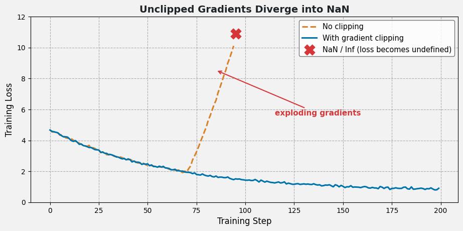
    (1) Exploding Gradients: Gradients grow without bound through many layers, producing weight updates so large that parameters overflow to Inf/NaN.
    (2) Unstable Math Operations: \log(0), division by zero, or square roots of negative numbers yield Inf/NaN. For example, batch normalization divides by zero variance if a batch is constant and no \epsilon is used.
    (3) Improper Learning Rate: A learning rate that is too high makes parameter updates diverge, pushing weights to extreme values that overflow.
    (4) Incorrect Weight Initialization: Initializing weights to very large values can overflow activations on the very first forward pass.
    (5) Data Issues: Inputs containing NaN, Inf, or extreme unnormalized values inject invalid numbers directly into the computation graph.

    Training loss curve where unclipped gradients explode and the loss becomes NaN, compared with stable training using gradient clipping.

    Figure 1: Unclipped gradients can explode within a few steps until the loss itself becomes NaN/Inf; gradient clipping keeps training on track.

    NaN Loss vs NaN Outputs: The two are stages of the same instability. A NaN loss can even appear while model outputs are still finite. For example, cross-entropy computes \log(\hat{y}), and a prediction extremely close to zero yields -\infty, which turns into NaN after the backward pass.

    Diagram of five common NaN causes with their standard fixes all feeding into NaN parameters and therefore NaN outputs.

    Figure 2: The five common causes and their standard fixes: every path ends at NaN parameters, hence NaN outputs.

    Mathematical Formulation:
    \mathcal{L} = -\log(\hat{y} + \epsilon)
    \hat{y} \to 0 \ \Rightarrow\ \mathcal{L} \to \infty \ \Rightarrow\ \text{NaN in backprop}
    g \leftarrow g \cdot \min\left(1,\ \frac{\tau}{\lVert g \rVert}\right)

    Where:

    • \hat{y} is the predicted probability of the true class; without the \epsilon clamp the loss diverges as \hat{y} approaches 0 and turns NaN in backprop.
    • g is the gradient vector and \tau the clipping threshold; the second rule (norm clipping) caps update magnitude before gradients can overflow the parameters.

    Login to view more content
  • DL0017 Reproducibility

    How do you ensure the reproducibility of deep learning experiments?

    Answer

    Reproducibility means a rerun of your experiment, by you or by someone else, produces the same results. Because deep learning pipelines are full of hidden randomness (weight initialization, data shuffling, dropout, GPU nondeterminism), achieving it requires controlling randomness with fixed seeds and deterministic operations, versioning code and configurations, pinning the software environment, fixing the dataset, and logging everything about each run.

    (1) Seed Control and Deterministic Operations: Fix random seeds for Python, NumPy, and your framework (PyTorch/TensorFlow), and enable deterministic algorithms while disabling autotuners that pick nondeterministic kernels.
    (2) Code and Configuration Versioning: Track code in Git and store every hyperparameter in versioned config files (YAML/JSON), so a run maps to an exact commit plus config.
    (3) Environment and Dependency Control: Pin library versions (requirements.txt, Conda) or containerize with Docker, recording CUDA/cuDNN and hardware details.
    (4) Dataset Management: Fix train/validation/test splits, document preprocessing, and use versioned datasets (e.g., DVC) so data never silently changes.
    (5) Logging and Experiment Tracking: Record seeds, configs, metrics, and artifacts for every run with tools like MLflow or Weights & Biases.

    What Failure Looks Like: Without seed control, two runs of identical code and data can trace visibly different accuracy curves (sometimes differing by a point or more at convergence), making results impossible to validate or compare.

    Two validation accuracy curves from identical code and data diverging because one run fixed its random seed and the other did not.

    Figure 1: Same code, same data, different curves: unseeded randomness alone is enough to make experiments non-reproducible.

    A Practical Pipeline: Treat reproducibility as a chain: each link below removes one source of variability, and the result is reproducible only if every link holds.

    Five-step reproducibility pipeline covering seed control, deterministic operations, code and config versioning, environment pinning, and data management with logging.

    Figure 2: Identical results require identical code + environment + data + seeds. A break in any link breaks the chain.

    Mathematical Formulation:
    m = F(\text{code},\ \text{config},\ \text{env},\ \text{data},\ \text{seed})
    \text{reproducible} \iff \forall\, i, j:\ m_i = m_j

    Where:

    • F is the full experiment pipeline viewed as a function of its five inputs; m is the resulting metric set (accuracy, loss curves).
    • m_i, m_j are metrics from any two reruns; reproducibility demands zero variance across runs, which holds only when all five inputs are fixed.

    Login to view more content
  • ML0047 Parameters

    What are the differences between parameters and hyperparameters?

    Answer

    Parameters are the values a model learns from its training data, while hyperparameters are settings defined by the user that guide the training process and model architecture. Parameters represent the model’s internal knowledge and decision rules; hyperparameters govern how the model learns, influencing its architecture, training dynamics, and ultimately its ability to generalize to unseen data: choosing them well is crucial for building an effective model.

    (1) Parameters: Internal variables learned from data (e.g., weights and biases); adjusted during training by the optimization algorithm; capture the model’s learned patterns and information.
    (2) Hyperparameters: External configurations set before training (e.g., learning rate, batch size, number of layers); remain fixed during training and are not updated by the learning process; influence how the model learns and its overall structure.
    (3) Who Updates Whom: The optimizer updates parameters by minimizing the loss; the practitioner (or a search procedure) updates hyperparameters by watching validation performance.

    Diagram contrasting parameters updated inside the training loop with hyperparameters set outside before training begins

    Figure 1: The two knobs of a model: parameters (weights, biases) live inside the training loop and are updated every step by the optimizer; hyperparameters (learning rate, batch size, depth, …) are set before training and shape how that loop behaves.

    Mathematical Formulation:
    \theta_{t+1} = \theta_t - \eta \, \nabla_\theta \mathcal{L}(\theta_t)
    \lambda^* = \arg\min_{\lambda} \; \mathcal{L}_{\text{val}}\big(\hat{\theta}(\lambda)\big)

    Where:

    • \theta denotes the parameters (weights and biases), updated every training step t by gradient descent.
    • \eta is the learning rate, itself a hyperparameter, set before training and never learned by the optimizer.
    • \lambda stands for hyperparameters generally; \hat{\theta}(\lambda) is the fully trained model under that setting, and the outer minimization over validation loss is hyperparameter search.

    Login to view more content
  • DL0016 Learning Rate Warmup

    What is learning rate warmup, and why does it help stabilize the early steps of deep network training?

    Answer

    Learning rate warmup starts training with a very small learning rate and increases it gradually (usually linearly) to the target peak over the first few hundred or thousand steps, after which the normal schedule (e.g., cosine decay) takes over. Its purpose is to stabilize early training: at initialization the model’s gradients are noisy and poorly conditioned, so immediately applying the full learning rate can cause loss spikes, divergence, or permanent damage to early layers.

    (1) Stabilizes Early Updates: Random initializations produce unreliable gradient estimates; small early steps prevent destructive weight changes before the model finds its footing.
    (2) Protects Adaptive Optimizers: With Adam, second-moment estimates are cold at step zero and can amplify the first updates; warmup bridges this biased-estimate phase.
    (3) Enables Higher Peak Rates: Deep networks and Transformers tolerate (and benefit from) a higher peak learning rate once representations have settled, which warmup makes reachable without instability.

    Learning rate schedule chart with a linear warmup from zero to a peak of 0.1 over 200 steps followed by a smooth cosine decay to zero by step 1000.

    Figure 1: A typical schedule: linear warmup for 200 steps to the 0.10 peak, then cosine decay to zero, the standard recipe behind models like BERT and GPT.

    Mathematical Formulation:
    \eta_t = \eta_{max} \cdot \frac{t}{T_{warm}}, \quad t \leq T_{warm}
    p = \frac{t - T_{warm}}{T - T_{warm}}
    \eta_t = \eta_{max} \cdot \tfrac{1}{2}\big(1 + \cos(\pi p)\big)

    Where:

    • \eta_t is the learning rate at step t; \eta_{max} is the target peak learning rate.
    • T_{warm} is the warmup length in steps (e.g., 200–10,000 depending on model and batch size).
    • T is the total number of training steps; after warmup, the schedule shown is cosine decay.
    • p \in [0, 1] is the post-warmup progress used by the third line, which applies once T_{warm} steps have elapsed: p = 0 at the end of warmup and p = 1 at the final step, so \eta_t decays from the peak to zero.

    Why It Matters in Practice: Transformers are famously sensitive: without warmup their early loss can spike or diverge outright, while warmup yields a smooth descent; the effect is smaller but still useful in CNN training at very large batch sizes.

    Training loss curves comparing stable training with warmup against a loss spike and divergence risk without warmup in the first sixty steps.

    Figure 2: Without warmup the early loss can spike and diverge; warmup keeps the fragile first steps small until gradients become trustworthy.


    Login to view more content
  • ML0046 Forward Propagation

    Please explain the process of Forward Propagation.

    Answer

    Forward propagation is the process by which a neural network takes an input and generates a prediction: the input data is passed systematically through each layer of the network. At every neuron, a weighted sum of the previous layer’s outputs (plus a bias) is computed, then a non-linear activation is applied; this repeats layer by layer until the output layer emits the final prediction. It is essentially the prediction phase of the network: information flows in one direction, from input to output, using the learned weights and biases.

    (1) Input Layer: The network receives the raw input data.
    (2) Layer-Wise Processing: Each neuron computes a linear combination (weighted sum plus bias), then applies a non-linear activation (ReLU, sigmoid, tanh) to introduce non-linearity.
    (3) Propagation Through Layers: The output of one layer becomes the input to the next, progressing through all hidden layers.
    (4) Output Generation: The final layer applies a task-appropriate function (softmax for classification, a linear function for regression) to produce the prediction.

    Forward propagation flow diagram showing inputs flowing through weighted sum, bias, and activation at each layer up to the output prediction

    Figure 1: One direction only: each layer transforms activations into pre-activations (z = Wx + b) and back into activations (a = f(z)) until the output layer produces the prediction. No gradient information flows here; that is backpropagation’s job.

    Mathematical Formulation:
    z^{(l)} = W^{(l)} a^{(l-1)} + b^{(l)}
    a^{(l)} = f\big(z^{(l)}\big)
    \hat{y} = a^{(L)}

    Where:

    • a^{(l-1)} is the previous layer’s activation vector (a^{(0)} = x, the input).
    • W^{(l)}, b^{(l)} are layer l‘s learned weights and biases; z^{(l)} is the pre-activation.
    • f(\cdot) is the activation function; L is the number of layers and \hat{y} the prediction.
    Small two three one network annotated with concrete input, weight, bias, pre-activation, and activation values flowing to a single numeric output

    Figure 2: A worked example with concrete numbers: inputs x = (0.5, 0.1, 0.4) flow through fixed weights and biases; each hidden node shows its computed z and sigmoid activation a, ending in the scalar prediction. Every number on the diagram follows from the two formulas above.


    Login to view more content
  • ML0045 Multi-Layer Perceptron

    What is a Multi-Layer Perceptron (MLP)? How does it overcome Perceptron limitations?

    Answer

    A Multi-Layer Perceptron (MLP) is a feedforward neural network with one or more hidden layers between the input and output layers. Its hidden layers use non-linear activation functions (ReLU, sigmoid, or tanh) to model complex relationships, and it is trained with backpropagation, which adjusts the weights to minimize errors. MLPs are used for classification, regression, and function approximation.

    (1) Hidden Layers + Non-Linearity: Each hidden unit applies a non-linear activation to its weighted sum, letting the network compose many linear maps into a curved function.
    (2) Overcomes The Perceptron: Unlike a single-layer perceptron (restricted to linearly separable problems), an MLP learns non-linear decision boundaries and handles problems such as XOR.
    (3) Universal Approximation: With enough neurons and layers, an MLP can approximate any continuous function, making it a powerful general-purpose model.

    MLP with four input nodes, two hidden layers of six and four nodes, and a three class output layer, fully connected

    Figure 1: An MLP for 3-class classification: 4 inputs, two hidden layers (6 and 4 units) with non-linear activations, and 3 softmax-style outputs. Every layer is fully connected to the next.

    Mathematical Formulation:
    h_l = f\big(W_l\, h_{l-1} + b_l\big)
    \hat{y} = g\big(W_L\, h_{L-1} + b_L\big)

    Where:

    • h_l is the activation vector of layer l (h_0 = x is the input).
    • W_l, b_l are the weight matrix and bias of layer l, learned by backpropagation.
    • f(\cdot) is the hidden non-linearity (ReLU/sigmoid/tanh); g(\cdot) is the output map (softmax for classification, identity for regression).
    XOR data with the single layer perceptron failing to separate it and the MLP carving a non-linear region that separates it

    Figure 2: The payoff: on XOR, the perceptron’s single line misclassifies half the positives, while the MLP’s hidden units carve a curved region that separates the classes perfectly.


    Login to view more content
  • ML0044 Perceptron

    Describe the Perceptron and its limitations.

    Answer

    The perceptron is a simple linear classifier that computes a weighted sum of input features, adds a bias, and applies a step function to produce a binary decision. It works well only for data that is linearly separable, where a straight line (or hyperplane in higher dimensions) can separate the classes.

    (1) Linear Score: The perceptron combines inputs linearly as w^T x + b; geometry-wise this defines one hyperplane.
    (2) Step Activation: A threshold turns the score into a hard 0/1 output. Note this non-linearity at the output still leaves the decision boundary linear.
    (3) Limitations: It cannot solve non-linearly-separable problems like XOR, a single layer cannot model complex patterns, and it outputs bare binary values with no confidence or probability.

    Perceptron diagram with three inputs and a constant one bias input feeding weighted arrows into a step activation output node

    Figure 1: Perceptron structure: inputs x_1, x_2, x_3 and a constant 1 (for the bias) feed through weights into a single unit whose step activation emits the binary output.

    Mathematical Formulation:
    y = f(w^T x + b)
    f(z) = 1 \text{ if } z \geq 0;\quad f(z) = 0 \text{ otherwise}

    Where:

    • y is the predicted output (0 or 1).
    • w is the weight vector, x the input vector, b the bias term.
    • f(\cdot) is the step activation; z = w^T x + b is the linear pre-activation whose sign alone decides the class.
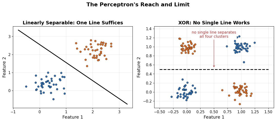
    Left panel linearly separable data split by one straight line, right panel XOR pattern that no single line can separate

    Figure 2: What one hyperplane can and cannot do: the left data is linearly separable and a perceptron solves it; the right XOR pattern defeats every single straight line, the classic motivation for hidden layers.


    Login to view more content
  • DL0015 Cold Start

    What is a “cold start” problem in deep learning?

    Answer

    The cold start problem is the difficulty of making reliable predictions for new entities (users, items, or contexts) that have little or no historical data. Models that depend on past interactions, especially recommender systems built on collaborative filtering, have no signal to learn a meaningful representation of a brand-new user or item, so their predictions degrade to near-random or popularity-biased guesses until data accumulates.

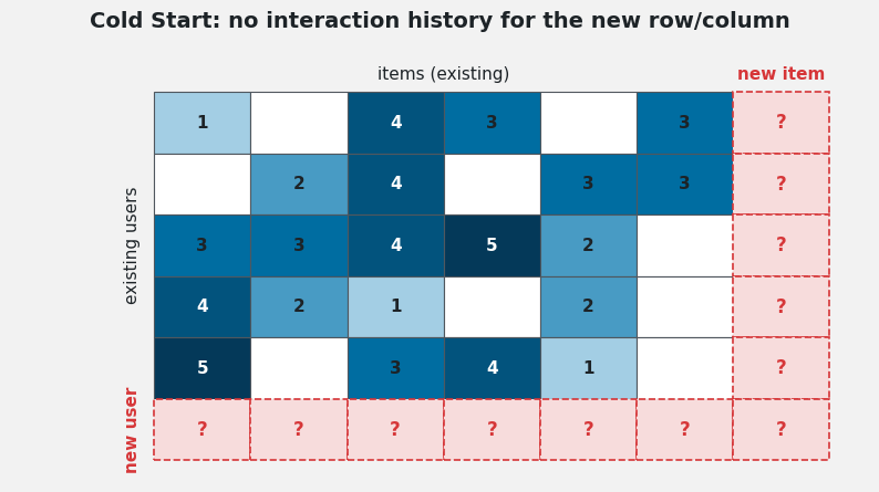
    (1) Missing Interaction History: Collaborative filtering infers taste from a user-item matrix; a new row (user) or column (item) is empty, so the model cannot locate the entity in its embedding space.
    (2) Feedback Loop Risk: Poor early predictions reduce engagement, which further slows data collection for the new entity. The problem compounds itself.
    (3) Three Flavors: New-user cold start, new-item cold start, and new-system cold start (no data at all) each demand different remedies.

    User-item rating matrix with observed ratings shaded by value and a dashed red new-user row and new-item column filled with question marks to illustrate the cold start problem.

    Figure 1: The new user row and new item column contain no interactions. Collaborative filtering has nothing to condition on for them.

    Mitigation Strategies: The common theme is supplying side information until interaction data accumulates: transfer learning borrows representations from related domains; hybrid models mix collaborative signals with content features; and active onboarding explicitly gathers a few preferences from new users.

    (1) Transfer Learning / Pre-trained Models: Initialize from embeddings or models trained on similar tasks so the new domain starts from useful structure rather than random weights.
    (2) Hybrid Recommendation Models: Combine collaborative filtering with content-based features (user demographics, item metadata) so predictions remain reasonable with zero interactions.
    (3) Active Learning / User Onboarding: Ask new users to rate a handful of popular or diverse items, turning cold start into a short warm-up phase.

    Diagram of three mitigation strategies, transfer learning, hybrid model, and active onboarding, feeding into a recommender that produces reasonable predictions for new users and items.

    Figure 2: All three strategies inject auxiliary signal into the recommender so cold entities get reasonable predictions before their interaction rows fill in.

    Mathematical Formulation:
    \hat{r}_{ui} = \mu + b_u + b_i + p_u^{\top} q_i

    Where:

    • \hat{r}_{ui} is the predicted rating of user u for item i; \mu is the global mean rating.
    • p_u and q_i are the learned latent factor vectors for user u and item i; b_u, b_i are bias terms.
    • Cold start means p_u or q_i was never trained: with an empty interaction row/column, the factors stay at random init, so \hat{r}_{ui} is meaningless.

    Login to view more content