Author: admin

ML0053 Hinge Loss for SVM
Explain the Hinge Loss function used in SVM.
Answer
The hinge loss is the key element of Support Vector Machines: it penalizes both misclassified points and correctly classified points that lie inside the margin. Points classified correctly with margin to spare get zero loss; the loss grows linearly as a point moves toward or across the decision boundary. This structure is exactly what pushes the SVM to maximize the margin, promoting robust, generalizable boundaries.
(1) Zero Loss Zone: When $y \cdot f(\mathbf{x}) \geq 1$ , the point is correctly classified and outside (or exactly on) the margin, the loss is 0.
(2) Linear Penalty Zone: When $y \cdot f(\mathbf{x})$ falls below 1, i.e., inside the margin or misclassified, the loss grows linearly with the violation.
(3) Convex But Not Smooth: The kink at $y \cdot f(\mathbf{x}) = 1$ makes the function non-differentiable there, so optimization uses subgradients instead of plain gradients.

Figure 1: Hinge loss vs the margin $y \cdot f(\mathbf{x})$ : flat at zero once the point is beyond the margin (right of the dashed line at 1), ramping up linearly inside the margin and for misclassified points (left of it). The kink at 1 is where subgradients take over.
Mathematical Formulation:
$\text{Hinge Loss} = \max\big(0,\; 1 - y \cdot f(\mathbf{x})\big)$
Where:
$y \in \{-1, +1\}$ is the true label.
$f(\mathbf{x})$ is the raw model output (the signed score, before any threshold).
The product $y \cdot f(\mathbf{x})$ is the (functional) margin: positive means correctly classified, ≥ 1 means correct with margin.
Login to view more content
June 11, 2025
ML0052 Non-Linear SVM
Can you explain the concept of a non-linear Support Vector Machine (SVM)?
Answer
A non-linear SVM classifies data that is not linearly separable by using a kernel function to implicitly project the data into a higher-dimensional space where a linear separator exists. This kernel trick provides flexibility for complex datasets while staying computationally efficient: the algorithm never computes the high-dimensional coordinates, only inner products through the kernel. The kernel choice (RBF, polynomial, sigmoid) strongly influences performance and adaptability.
(1) Kernel Trick: Replace inner products with a kernel $K(\mathbf{x}_i, \mathbf{x}_j)$ , which measures similarity as if the data were mapped to a higher-dimensional space, where a linear separation becomes possible.
(2) Common Kernels: Polynomial (captures feature interactions of degree $d$ ), RBF/Gaussian (local similarity decaying with distance), sigmoid (imitates a neural activation).
(3) Objective: Find the margin-maximizing hyperplane in the transformed space; in the original space its image is a curved decision boundary.

Figure 1: Same data, two SVMs: the linear kernel can only slice the moons with a straight line (left), while the RBF kernel’s implicit high-dimensional map lets the boundary bend around both crescents (right).
Mathematical Formulation:
$K(\mathbf{x}_i, \mathbf{x}_j) = (\gamma\, \mathbf{x}_i^\top \mathbf{x}_j + c)^d$
$K(\mathbf{x}_i, \mathbf{x}_j) = \exp\big(-\gamma \|\mathbf{x}_i - \mathbf{x}_j\|^2\big)$
$K(\mathbf{x}_i, \mathbf{x}_j) = \tanh(\gamma\, \mathbf{x}_i^\top \mathbf{x}_j + c)$
Where (polynomial, RBF, sigmoid kernels in order):
$\mathbf{x}_i, \mathbf{x}_j$ are input vectors; $\gamma$ scales the inner product or controls the RBF width ( $\gamma = 1/(2\sigma^2)$ , with $\sigma$ the Gaussian spread).
$c$ is a constant (bias) term and $d$ the polynomial degree.
$\|\mathbf{x}_i - \mathbf{x}_j\|^2$ is the squared Euclidean distance: nearby points get RBF similarity near 1, distant points near 0.

Figure 2: The kernel idea made concrete: in 1-D the blue class sits between the oranges and no single threshold separates them; after the explicit lift $x \mapsto (x, x^2)$ the classes part vertically and one straight line suffices. Kernels compute as if this lift happened, without ever forming the new coordinates.
Login to view more content
June 11, 2025
ML0051 Linear SVM
Can you explain the key concepts behind a Linear Support Vector Machine?
Answer
A Linear Support Vector Machine (Linear SVM) is a classifier that finds the optimal straight line (hyperplane) separating two classes by maximizing the margin between them. It relies on a few critical points (the support vectors) and offers strong generalization, especially on linearly separable data.
(1) Hyperplane: The decision boundary that separates data points of different classes.
(2) Margin: The distance between the hyperplane and the nearest data point of each class; the SVM maximizes it.
(3) Support Vectors: The points lying closest to the hyperplane; they alone define it: moving any other point changes nothing.
(4) Objective: Maximize the margin while minimizing classification error (hard margin forbids error; soft margin prices it in).

Figure 1: Hard-margin SVM: the solid hyperplane $w^T x + b = 0$ sits midway between the dashed margins $w^T x + b = \pm 1$ , and only the circled support vectors touch the margin: they alone determine the boundary.
Mathematical Formulation:
$f(\mathbf{x}) = \mathbf{w}^\top \mathbf{x} + b$
$\hat{y} = \mathrm{sign}(\mathbf{w}^\top \mathbf{x} + b) = \mathrm{sign}(f(\mathbf{x}))$
$\min_{\mathbf{w}, b} \; \frac{1}{2} \|\mathbf{w}\|^2$
$\text{subject to } y_i(\mathbf{w}^\top \mathbf{x}_i + b) \geq 1 \quad \text{for all } i$
Where:
$\mathbf{x}$ is the input feature vector, $\mathbf{w}$ the weight vector, $b$ the bias; $\hat{y}$ is the predicted label.
$\mathrm{sign}(\cdot)$ returns +1 if its argument is ≥ 0 and −1 otherwise; $y_i \in \{-1, +1\}$ is the true label of point $\mathbf{x}_i$ .
Minimizing $\frac{1}{2}\|\mathbf{w}\|^2$ under those constraints is the hard-margin objective: since the margin width is $2 / \|\mathbf{w}\|$ , small $\|\mathbf{w}\|$ means a wide margin.
Login to view more content
June 11, 2025
ML0050 Logistic Regression III
Why is Mean Squared Error (L2 Loss) an unsuitable loss function for logistic regression compared to cross-entropy?
Answer
Mean Squared Error (MSE) is unsuitable for logistic regression primarily because, combined with the sigmoid, it produces a non-convex loss landscape: optimization becomes harder and convergence less reliable. It also provides weaker gradients exactly when predictions are confidently wrong, slowing learning. Cross-entropy aligns with the Bernoulli distribution assumption behind binary classification, yields a convex loss for the single-neuron binary setting, and delivers strong gradients throughout.
(1) Wrong Assumption: MSE assumes Gaussian-distributed errors, while logistic regression models a Bernoulli (binary) outcome.
(2) Non-Convex Optimization: MSE on top of the sigmoid creates a non-convex surface: gradient descent can stall in flat regions or poor local behavior.
(3) Gradient Issues: With MSE, confident wrong predictions produce tiny gradients (the sigmoid saturates), slowing learning; cross-entropy keeps the gradient strong precisely there.
(4) Interpretation: Cross-entropy directly compares predicted probabilities to true labels, the natural measure for classification.

Figure 1: The MSE loss surface over $(w, b)$ for a sigmoid classifier: wide, nearly flat plateaus (vanishing gradients where the sigmoid saturates) around a narrow curved valley: a landscape that is awkward and slow for gradient descent, unlike the convex bowl cross-entropy gives.
Mathematical Formulation:
$\mathcal{L}_{\text{MSE}} = \frac{1}{n} \sum_{i=1}^{n} \big(y_i - \sigma(z_i)\big)^2$
$\mathcal{L}_{\text{CE}} = -\frac{1}{n} \sum_{i=1}^{n} \Big[ y_i \log \sigma(z_i) + (1 - y_i) \log \big(1 - \sigma(z_i)\big) \Big]$
$\frac{\partial \mathcal{L}_{\text{CE}}}{\partial z_i} = \sigma(z_i) - y_i$
Where:
$y_i \in \{0, 1\}$ is the true label and $\sigma(z_i)$ the predicted probability for sample $i$ , with score $z_i = \mathbf{w}^{\top}\mathbf{x}_i + b$ .
MSE’s gradient carries an extra factor $\sigma'(z_i) = \sigma(z_i)(1 - \sigma(z_i))$ , which vanishes when the sigmoid saturates, exactly when the prediction is confidently wrong.
Cross-entropy’s gradient $\sigma(z_i) - y_i$ is simply the prediction error: large when the model is confidently wrong, with no saturating factor.
Login to view more content
June 10, 2025

ML0049 Logistic Regression II

Please compare Logistic Regression and Neural Networks.

Answer

Logistic regression is a straightforward, linear model suited to linearly separable data, offering good interpretability and fast, simple training. Neural networks are powerful non-linear models capable of capturing intricate patterns in large datasets, often at the expense of interpretability and higher computational demands.

(1) Expressiveness: Logistic regression draws one hyperplane; neural networks compose hidden layers into arbitrarily curved boundaries.
(2) Workflow: Logistic regression often needs manual feature engineering; neural networks learn feature representations automatically.
(3) Cost: Logistic regression trains in seconds with low overfitting risk when features are well chosen; networks need more data, compute, and regularization.

Logistic regression drawn as a neural network with an input layer feeding one sigmoid output neuron, with no hidden layer

Figure 1: Logistic regression is a neural network: an input layer plus a single output neuron with a sigmoid activation and no hidden layer, the simplest possible network, for binary classification.

Mathematical Formulation:
$\hat{y} = \sigma(\mathbf{w}^{\top} \mathbf{x} + b)$
$\hat{y} = g\big(W_L \, f(\cdots f(W_1 \mathbf{x} + b_1) \cdots) + b_L\big)$

Where:

The first line is logistic regression: one linear score through a sigmoid $\sigma$ , equivalent to a 0-hidden-layer network.
The second line is a general neural network: compositions of weight matrices $W_l$ , biases $b_l$ , and non-linearities $f$ , with output map $g$ .
Setting the number of hidden layers to zero and $g = \sigma$ recovers logistic regression exactly.

Feature	Logistic Regression	Neural Networks (NN)
Model Type	Linear	Non-linear, multi-layer
Architecture	Single-layer (no hidden layers)	Multi-layer (can be deep)
Non-linearity	Can’t model non-linear relationships directly	Can capture complex non-linear patterns
Feature Engineering	Often needed manually	Learns feature representations automatically
Interpretability	High	Low (acts like a black box)
Training Time	Fast, simple to train	Slower, needs more compute & data
Overfitting Risk	Low (if features are well-chosen)	Higher (requires regularization)
Common Use Cases	Simple classification problems (e.g., churn prediction)	Complex tasks (e.g., image, text, speech recognition)

June 10, 2025

ML0048 Logistic Regression

Can you explain logistic regression and how it contrasts with linear regression?

Answer

Logistic regression maps inputs to a probability space for classification, while linear regression estimates continuous outcomes through a direct linear relationship. Logistic regression estimates the probability that a binary outcome ( $y = 1$ ) occurs given an input vector $\mathbf{x}$ , by passing a linear score through the sigmoid function; the output lies between 0 and 1 and is interpreted as the probability of class membership. Note that standard logistic regression is still fundamentally a linear model at its core: it cannot model non-linear relationships directly.

(1) Purpose: Linear regression predicts a continuous output (price, height); logistic regression predicts a probability for classification (spam or not).
(2) Output Range: Linear regression emits any real number (can be negative or above 1); logistic regression squashes to (0, 1) with the sigmoid.
(3) Assumption: Linear regression assumes a linear input-output relationship; logistic regression assumes a linear relationship between inputs and the log-odds of the positive class.

Left panel linear regression line fitting continuous data, right panel sigmoid curve fitting binary zero one data with a 0.5 decision boundary

Figure 1: The contrast in one picture: linear regression fits a straight line through continuous targets (left); logistic regression fits an S-shaped sigmoid to 0/1 labels (right), with the 0.5 probability level acting as the decision boundary.

Mathematical Formulation:
$\Pr(y = 1 \mid \mathbf{x}) = \frac{1}{1 + e^{-(\mathbf{w}^{\top} \mathbf{x} + b)}}$

Where:

$\mathbf{x}$ is the input feature vector.
$\mathbf{w}$ is the weight vector and $b$ the bias; the linear score $\mathbf{w}^{\top}\mathbf{x} + b$ is the log-odds of the positive class.
The sigmoid maps the score to (0, 1); classifying at threshold 0.5 gives a linear decision boundary.

Feature	Logistic Regression	Linear Regression
Type of Problem	Classification	Regression
Dependent Variable	Categorical (e.g., Yes/No, 0/1, True/False)	Continuous (e.g., Price, Temperature, Age)
Output	Probability (0 to 1)	Real number (any value)
Core Function	Sigmoid function (for binary)	Identity function
Loss Function	Log-loss (Cross-entropy)	Mean Squared Error (MSE)

June 9, 2025

DL0024 Fixed-size Input in CNN
What is the “dilemma of fixed-size input” for CNNs? How is it typically resolved?
Answer
The dilemma of fixed-size input is the constraint that classic CNN classifiers (VGG, early ResNets) only accept images of one predetermined resolution: the fully connected head has a weight matrix whose input dimension equals the flattened feature-map size, and that size is only constant if every input image has the same $H \times W$ . Real-world images arrive in arbitrary sizes, so they must be resized or cropped first, distorting aspect ratios, discarding small objects, or cutting content away.
(1) The FC Head Is the Bottleneck: Convolutions themselves handle any spatial size; only the flatten + FC stage pins the input dimensions.
(2) Preprocessing Costs Information: Resizing squishes content and can erase small objects; cropping keeps resolution but discards everything outside the window.
(3) Structural Fixes Exist: Replace or decouple the FC head (GAP, fully convolutional designs, or adaptive pooling) and the network accepts variable sizes natively.

Figure 1: Both standard fixes hurt: downsampling erases small objects; cropping amputates anything near the border.
Mathematical Formulation (Why the FC Head Fixes the Size):
$z = W \cdot \mathrm{vec}(X) + b, \quad X \in \mathbb{R}^{H \times W \times C}$
$\mathrm{GAP}(X)_c = \frac{1}{HW} \sum_{h=1}^{H} \sum_{w=1}^{W} X_{hwc}$
Where:
$X$ is the final feature volume; $\mathrm{vec}(X)$ flattens it to $HWC$ values, so $W$ exists only for one specific $H \times W$ .
$\mathrm{GAP}(X)_c$ averages channel $c$ over all spatial positions, yielding a $C$ -dimensional vector for any input size.
Common Solutions: (1) Global Average Pooling: replace the flatten with a per-channel average, so the classifier sees exactly $C$ values regardless of resolution; (2) Fully Convolutional Networks: remove FC layers entirely and let the output scale with the input (standard for segmentation); (3) Adaptive Pooling: pool to a fixed $k \times k$ grid no matter the input size (e.g., nn.AdaptiveAvgPool2d in PyTorch).

Figure 2: Three structural escapes (GAP, FCN, and adaptive pooling) all remove the fixed-size constraint at its source: the FC head.
Login to view more content
June 8, 2025
DL0023 Dilated Convolution
What are dilated convolutions? When would you use them?
Answer
Dilated convolutions (also called atrous convolutions) insert gaps between the elements of a convolutional kernel: with dilation rate $d$ , the kernel samples every $d$ -th input position instead of adjacent ones. This expands the receptive field without adding parameters and without reducing spatial resolution, a combination that pooling cannot offer. A dilation rate of 1 is just a standard convolution.
(1) Larger Receptive Field, Same Weights: A 3×3 kernel with dilation 2 covers a 5×5 area but still has only 9 weights.
(2) Resolution Preserved: Unlike pooling, dilation grows the receptive field while keeping the output the same size as a standard convolution, which is critical for dense prediction.
(3) Multi-Scale Context: Stacking or mixing dilation rates lets one network aggregate both fine local detail and broad context.

Figure 1: Same 3 weights, wider view: dilation 3 spreads the taps across a receptive field of 7 instead of 3.
Mathematical Formulation:
$y_{ij} = \sum_{a=1}^{k}\sum_{b=1}^{k} w_{ab}\; x_{i + d \cdot a,\; j + d \cdot b}$
$k_{eff} = k + (k - 1)(d - 1)$
Where:
$d$ is the dilation rate, the spacing between tapped positions ( $d = 1$ is standard convolution).
$k$ is the nominal kernel size; $k_{eff}$ is the effective span of the dilated kernel (3×3 with $d = 2$ behaves like 5×5 with holes).
$w_{ab}$ are the kernel weights; the parameter count is independent of $d$ .
In Two Dimensions: The same idea applies to images: the kernel’s taps spread over a checkerboard-like stencil, expanding the covered span from 3×3 to 5×5 at dilation 2 while the channel count and output resolution stay unchanged.

Figure 2: Dilation 2 turns a 3×3 stencil into a 5×5 receptive field (red dashed box), still only 9 multiply-accumulates.
When to Use Them: Any task needing large context at full resolution: semantic segmentation (DeepLab), audio generation (WaveNet models long-range temporal structure with exponentially growing dilation), and dense tasks like super-resolution or depth estimation.

Figure 3: Gridding artifacts: stacking the same dilation leaves a checkerboard of unattended cells. Mitigate with hybrid dilation rates (e.g., 1, 2, 5) that overlap coverage.
Login to view more content
May 31, 2025
DL0022 CNN Architecture
Describe the typical architecture of a CNN.
Answer
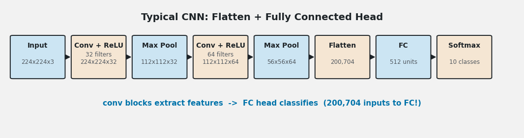
A typical Convolutional Neural Network chains together a small set of repeating building blocks: the raw input passes through stacked convolution + activation layers that extract local features, interleaved with pooling layers that halve the spatial resolution, after which the feature maps are flattened (or globally pooled) and fed into fully connected layers ending in a softmax output for classification. Regularizers such as dropout and batch normalization are commonly inserted along the way.
(1) Feature Extraction Front-End: Repeated conv → ReLU → pool blocks build hierarchical features while shrinking spatial size and growing channels.
(2) Classification Head: Flattened features (or a GAP vector) feed fully connected layers that combine features into class scores.
(3) Output Layer: Softmax for multi-class, sigmoid for binary/multi-label; optional dropout, batch norm, and skip connections stabilize training.

Figure 1: The canonical pipeline: spatial size shrinks (224 → 112 → 56) while channels grow (3 → 32 → 64), then a flatten + FC head classifies. Note the 200,704 values hitting the FC layer.
Mathematical Formulation:
$W_{out} = \left\lfloor \frac{W_{in} - k + 2p}{s} \right\rfloor + 1$
$P(y = i \mid z) = \frac{e^{z_i}}{\sum_{j=1}^{K} e^{z_j}}$
Where:
$W_{in}, W_{out}$ are the input and output spatial sizes of a conv or pool layer; $k$ is the kernel size, $p$ the padding, $s$ the stride.
$z_i$ is the logit for class $i$ ; $K$ is the number of classes; the softmax converts logits into a probability distribution.
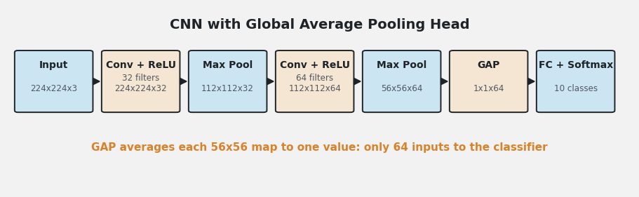
Modern Variant: GAP Head: Many modern CNNs (ResNet, MobileNet) replace the flatten + large FC head with Global Average Pooling, which averages each feature map to a single number before a small classifier. This slashes parameters, removes the fixed-input constraint, and reduces overfitting.

Figure 2: Swapping flatten for GAP shrinks the classifier input from 200,704 to 64 values, millions fewer parameters in the head.
Login to view more content
May 31, 2025
DL0021 Feature Map
What is the feature map in Convolutional Neural Networks?
Answer
A feature map is the output produced when one convolutional filter slides across its input: a 2D grid of activations whose values encode where and how strongly a specific pattern (an edge orientation, texture, or object part) appears at each spatial location. A convolutional layer applies many filters in parallel, so its output is a stack of feature maps, one per filter, forming the layer’s channels.
(1) Output of One Filter: Each feature map is generated by a single filter convolving over the input; the layer output stacks one map per filter, so 64 filters produce 64 channels.
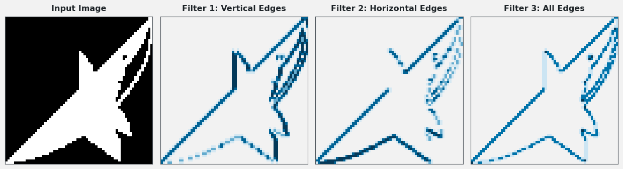
(2) Location and Strength: A high activation at position (i, j) means the filter’s pattern (e.g., a vertical edge or a corner) is strongly present around that location.
(3) Evolving Semantics with Depth: Early maps respond to edges and textures, middle maps to parts and shapes, and deep maps to whole objects with class-specific meaning.

Figure 1: Three filters applied to the same input produce three different feature maps; each lights up where its own pattern (vertical, horizontal, or any edge) appears.
Mathematical Formulation:
$y^{(c)}_{ij} = \sum_{a=1}^{k}\sum_{b=1}^{k}\sum_{d=1}^{C_{in}} w^{(c)}_{abd}\, x_{i+a,\, j+b,\, d} + b_c$
$\text{output shape} = (H_{out},\ W_{out},\ C_{out}), \quad C_{out} = \text{number of filters}$
Where:
$y^{(c)}_{ij}$ is the activation of feature map $c$ at spatial position $(i, j)$ .
$w^{(c)}_{abd}$ are the weights of filter $c$ of size $k \times k \times C_{in}$ ; $b_c$ is its bias.
$x_{i+a,\, j+b,\, d}$ is the input activation; $C_{in}$ and $C_{out}$ are the input and output channel counts.
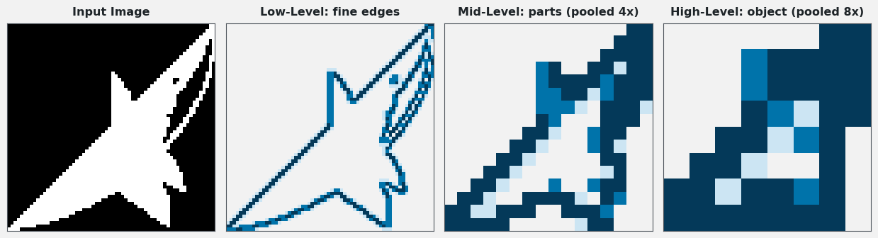
Hierarchical Representation: As activations flow deeper, each new feature map is computed from the previous layer’s maps, so neurons see progressively larger receptive fields and combine simpler patterns into richer ones, the foundation of a CNN’s representational power.

Figure 2: Depth turns fine edges into parts and finally into an object-level representation. Resolution drops while semantic content rises.
Login to view more content
May 31, 2025