Category: Medium

  • ML0058 K-means++

    Please explain how K-means++ works.

    Answer

    K-means++ is an improved way to initialize the centroids of K-means. Instead of picking all centroids uniformly at random, it selects them one by one with probability proportional to the squared distance from the already chosen centroids. This spreads the initial centroids out, sharply reducing the chance of poor clustering and helping the algorithm converge faster and more reliably. After initialization, standard K-means proceeds unchanged.

    (1) First Centroid: Choose \mu_1 uniformly at random from the dataset.
    (2) Distance Computation: For each point, compute its squared distance to the nearest already-chosen centroid.
    (3) Weighted Selection: Pick the next centroid with probability proportional to that squared distance: far points are favored.
    (4) Repeat Until K: Continue until all K centroids are chosen, then run standard K-means.

    Five clusters with centroids initialized by K-means plus plus landing one per cluster

    Figure 1: K-means++ initialization (K=5): the distance-squared weighting spreads the starting centroids across all five natural groups, so the algorithm starts close to a good solution instead of gambling on random seeds.

    Mathematical Formulation:
    D(x_i)^2 = \min_{1 \le j \le m} \|x_i - \mu_j\|^2
    P(x_i) = \frac{D(x_i)^2}{\sum_j D(x_j)^2}

    Where:

    • \mu_j is one of the m already chosen centroids; D(x_i)^2 is point x_i‘s squared distance to its nearest chosen centroid.
    • P(x_i) is the probability of x_i becoming the next centroid, proportional to D(x_i)^2, so points far from every chosen centroid are exponentially favored over nearby ones.
    • The denominator normalizes over all data points; selection repeats until K centroids exist.
    Side by side comparison where random initialization merges two groups and splits one while K-means plus plus finds all three true clusters

    Figure 2: Why initialization matters: with an unlucky random init (left), two centroids land in one group and the small top cluster is merged away; K-means++ (right) seeds one centroid per group and recovers all three clusters cleanly.

    Login to view more content
  • ML0056 K Selection in KNN

    In the context of designing a K-Nearest Neighbors (KNN) model, can you explain your approach to selecting the value of K?

    Answer

    Selecting K in KNN is crucial because it directly controls model performance through the bias-variance tradeoff. The systematic approach is k-fold cross-validation combined with grid search over a range of K values, picking the one that minimizes validation error, informed where possible by domain knowledge and data characteristics.

    (1) Bias-Variance Tradeoff: A small K (e.g., 1) gives low bias but high variance: it tracks noise and overfits; a large K raises bias but lowers variance: it oversmooths and can underfit.
    (2) Use Odd Values For Classification: In binary classification, an odd K avoids tie votes.
    (3) Cross-Validation + Grid Search: Evaluate every candidate K with k-fold CV and select the minimizer of validation error.
    (4) Domain Knowledge: Prior knowledge of the data distribution can narrow the search range.

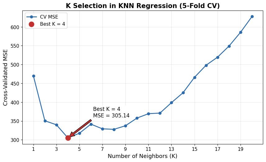
    Cross validated MSE curve over K from 1 to 20 with a minimum marked at K equals 4

    Figure 1: 5-fold CV error across K on a regression task: error dives as variance is tamed (tiny K overfits), bottoms at K = 4, then climbs steadily as over-averaging sets in (large K underfits). The minimizer is the selected K.

    Mathematical Formulation:
    CV(K) = \frac{1}{N} \sum_{i=1}^{N} \ell\big(y_i, \hat{y}_i(K)\big)

    Where:

    • y_i is the actual outcome for the i-th validation instance.
    • \hat{y}_i(K) is the prediction made using K neighbors (with the point’s own fold held out).
    • N is the number of validation samples and \ell the loss (e.g., squared error for regression, 0-1 for classification).

    Login to view more content
  • ML0052 Non-Linear SVM

    Can you explain the concept of a non-linear Support Vector Machine (SVM)?

    Answer

    A non-linear SVM classifies data that is not linearly separable by using a kernel function to implicitly project the data into a higher-dimensional space where a linear separator exists. This kernel trick provides flexibility for complex datasets while staying computationally efficient: the algorithm never computes the high-dimensional coordinates, only inner products through the kernel. The kernel choice (RBF, polynomial, sigmoid) strongly influences performance and adaptability.

    (1) Kernel Trick: Replace inner products with a kernel K(\mathbf{x}_i, \mathbf{x}_j), which measures similarity as if the data were mapped to a higher-dimensional space, where a linear separation becomes possible.
    (2) Common Kernels: Polynomial (captures feature interactions of degree d), RBF/Gaussian (local similarity decaying with distance), sigmoid (imitates a neural activation).
    (3) Objective: Find the margin-maximizing hyperplane in the transformed space; in the original space its image is a curved decision boundary.

    Two panels on interleaving moons data showing the linear SVM's straight boundary cutting through a class and the RBF SVM's curved boundary separating them cleanly

    Figure 1: Same data, two SVMs: the linear kernel can only slice the moons with a straight line (left), while the RBF kernel’s implicit high-dimensional map lets the boundary bend around both crescents (right).

    Mathematical Formulation:
    K(\mathbf{x}_i, \mathbf{x}_j) = (\gamma\, \mathbf{x}_i^\top \mathbf{x}_j + c)^d
    K(\mathbf{x}_i, \mathbf{x}_j) = \exp\big(-\gamma \|\mathbf{x}_i - \mathbf{x}_j\|^2\big)
    K(\mathbf{x}_i, \mathbf{x}_j) = \tanh(\gamma\, \mathbf{x}_i^\top \mathbf{x}_j + c)

    Where (polynomial, RBF, sigmoid kernels in order):

    • \mathbf{x}_i, \mathbf{x}_j are input vectors; \gamma scales the inner product or controls the RBF width (\gamma = 1/(2\sigma^2), with \sigma the Gaussian spread).
    • c is a constant (bias) term and d the polynomial degree.
    • \|\mathbf{x}_i - \mathbf{x}_j\|^2 is the squared Euclidean distance: nearby points get RBF similarity near 1, distant points near 0.
    Left panel one dimensional class data not separable by a point, right panel the same data lifted to two dimensions by x squared mapping and separated by a straight line

    Figure 2: The kernel idea made concrete: in 1-D the blue class sits between the oranges and no single threshold separates them; after the explicit lift x \mapsto (x, x^2) the classes part vertically and one straight line suffices. Kernels compute as if this lift happened, without ever forming the new coordinates.


    Login to view more content
  • ML0050 Logistic Regression III

    Why is Mean Squared Error (L2 Loss) an unsuitable loss function for logistic regression compared to cross-entropy?

    Answer

    Mean Squared Error (MSE) is unsuitable for logistic regression primarily because, combined with the sigmoid, it produces a non-convex loss landscape: optimization becomes harder and convergence less reliable. It also provides weaker gradients exactly when predictions are confidently wrong, slowing learning. Cross-entropy aligns with the Bernoulli distribution assumption behind binary classification, yields a convex loss for the single-neuron binary setting, and delivers strong gradients throughout.

    (1) Wrong Assumption: MSE assumes Gaussian-distributed errors, while logistic regression models a Bernoulli (binary) outcome.
    (2) Non-Convex Optimization: MSE on top of the sigmoid creates a non-convex surface: gradient descent can stall in flat regions or poor local behavior.
    (3) Gradient Issues: With MSE, confident wrong predictions produce tiny gradients (the sigmoid saturates), slowing learning; cross-entropy keeps the gradient strong precisely there.
    (4) Interpretation: Cross-entropy directly compares predicted probabilities to true labels, the natural measure for classification.

    Three dimensional MSE loss surface over weight and bias for logistic regression showing flat plateaus and a narrow steep valley

    Figure 1: The MSE loss surface over (w, b) for a sigmoid classifier: wide, nearly flat plateaus (vanishing gradients where the sigmoid saturates) around a narrow curved valley: a landscape that is awkward and slow for gradient descent, unlike the convex bowl cross-entropy gives.

    Mathematical Formulation:
    \mathcal{L}_{\text{MSE}} = \frac{1}{n} \sum_{i=1}^{n} \big(y_i - \sigma(z_i)\big)^2
    \mathcal{L}_{\text{CE}} = -\frac{1}{n} \sum_{i=1}^{n} \Big[ y_i \log \sigma(z_i) + (1 - y_i) \log \big(1 - \sigma(z_i)\big) \Big]
    \frac{\partial \mathcal{L}_{\text{CE}}}{\partial z_i} = \sigma(z_i) - y_i

    Where:

    • y_i \in \{0, 1\} is the true label and \sigma(z_i) the predicted probability for sample i, with score z_i = \mathbf{w}^{\top}\mathbf{x}_i + b.
    • MSE’s gradient carries an extra factor \sigma'(z_i) = \sigma(z_i)(1 - \sigma(z_i)), which vanishes when the sigmoid saturates, exactly when the prediction is confidently wrong.
    • Cross-entropy’s gradient \sigma(z_i) - y_i is simply the prediction error: large when the model is confidently wrong, with no saturating factor.

    Login to view more content
  • ML0033 All Zeros Init

    How does initializing all weights and biases to zero affect a neural network’s training?

    Answer

    Initializing every weight and bias to zero creates a fatal symmetry problem: all neurons in a layer compute the same output, receive the same gradient, and update identically, so they remain identical forever. The layer effectively behaves as a single neuron no matter how wide it is, the network cannot learn diverse features, and its representational capacity collapses. The pathology goes further: with zero weights, activations propagate as zero through the layers (for ReLU the forward signal is exactly 0), and gradients backpropagating through zero weights vanish entirely, so training can stall from the very first step. Proper initialization is therefore not a cosmetic choice: random schemes like Xavier/He break the symmetry and set the activation scale so signals flow through the full depth of the network.

    (1) Symmetry: Identical weights → identical outputs → identical gradients → identical neurons forever; width is wasted.
    (2) No Learning Signal: Zero weights kill forward activations and backward gradients (especially with ReLU), stalling training.
    (3) Fix: Small random initialization (Xavier/He) breaks symmetry and keeps activation/gradient variance stable across layers.

    Training and validation accuracy for zero initialization stuck at chance level versus random initialization learning successfully

    Figure 1: Zero versus random initialization on a binary task: with all-zero weights, train and validation accuracy stay pinned at the 0.5 chance level: the network learns nothing; random initialization breaks symmetry and both curves climb above 0.9.

    Mathematical Formulation:
    z_j = \sum_{i} w_{ji} x_i + b_j = 0 \quad \forall j \;\; (\text{all-zero init})
    \frac{\partial L}{\partial w_{ji}} = \delta_j \, x_i
    \delta_j = f'(z_j) \sum_k \delta_k w_{kj} = 0

    Where:

    • w_{ji} is the weight from input i to neuron j, b_j its bias, z_j its pre-activation.
    • \delta_j is the backpropagated error signal of neuron j; with downstream weights w_{kj} = 0 it collapses to 0, so every weight gradient is 0.
    • Even where a gradient exists (first layer before the collapse), every neuron in a layer gets the same gradient and stays identical: the symmetry itself is the deeper failure.

    Login to view more content
  • ML0029 Tanh

    What are the advantages and disadvantages of using the tanh activation function?

    Answer

    The tanh (hyperbolic tangent) activation squashes its input into the range (-1, 1) with a smooth S-shape. Its headline advantage over sigmoid is that its output is zero-centered: activations average near zero, so the gradients flowing into the next layer do not systematically push all weights in one direction, which makes optimization easier and convergence faster. It is also smooth and infinitely differentiable, and its maximum derivative of 1 (versus sigmoid’s 0.25) gives stronger gradients near the active region. The disadvantages are the flip side of saturation: for large positive or negative inputs the function flattens and its derivative approaches zero, so deep stacks of tanh units suffer the vanishing gradient problem; and like sigmoid it requires exponentials, making it computationally more expensive than ReLU. Because its output is not in (0, 1), it is also unsuitable as a probability output; its modern niche is mainly inside RNN/LSTM cell dynamics rather than feedforward hidden layers.

    (1) Zero-Centered: Output range (-1, 1) centers activations, easing optimization versus sigmoid’s all-positive outputs.
    (2) Stronger Gradient: Maximum derivative 1 at the origin (4× sigmoid’s), but it still saturates in the tails.
    (3) Costs: Vanishing gradients in deep stacks, exponential computation, and no probability interpretation of the output.

    Tanh curve between minus one and one with its derivative peaking at one and vanishing in the tails

    Figure 1: Tanh and its derivative 1 - \tanh^2(x): the zero-centered S-curve has a healthy gradient (peak 1) only in the narrow central region; in both tails the derivative collapses toward zero.

    Mathematical Formulation:
    \tanh(x) = \frac{e^{x} - e^{-x}}{e^{x} + e^{-x}} = 2\,\sigma(2x) - 1
    \frac{d}{dx}\tanh(x) = 1 - \tanh^2(x) \in (0, 1]

    Where:

    • x is the neuron’s pre-activation; \sigma(\cdot) is the logistic sigmoid, showing tanh is just a rescaled sigmoid.
    • 1 - \tanh^2(x) is the derivative: maximal (1) at x = 0, decaying toward 0 as |x| grows, the saturation that drives vanishing gradients.

    Login to view more content
  • ML0027 Leaky ReLU

    What are the benefits of the Leaky ReLU activation function?

    Answer

    Leaky ReLU modifies standard ReLU by replacing the hard zero on the negative side with a small linear slope: negative inputs pass through scaled by a small constant \alpha (typically 0.01). This one change directly attacks ReLU’s main weakness: the dying ReLU problem. Because the negative region now carries a small but non-zero gradient, a neuron whose pre-activation goes negative for all inputs still receives learning signal and can be pulled back into the active regime, instead of being frozen at zero output forever. At the same time Leaky ReLU retains everything that made ReLU attractive: the positive side stays the identity with gradient 1 (no vanishing gradients), the computation is still a trivial piecewise-linear threshold, and the output remains unbounded above, preserving ReLU’s scale behavior. In practice the accuracy gain over ReLU is often modest, but it costs nothing and removes a permanent failure mode.

    (1) Fixes Dying ReLU: Negative inputs get slope \alpha instead of 0, so gradient always flows and “dead” neurons can recover.
    (2) Keeps ReLU’s Strengths: Identity on the positive side (gradient 1, no saturation) and near-identical computational cost.
    (3) Costs: Introduces the hyperparameter \alpha (or learns it, as in PReLU); practical accuracy gains over ReLU are often small.

    ReLU versus Leaky ReLU curves with the small negative slope highlighted

    Figure 1: ReLU versus Leaky ReLU: identical on the positive side, but Leaky ReLU keeps a small slope \alpha in the negative region, enough gradient for a stuck neuron to recover instead of dying.

    Mathematical Formulation:
    \mathrm{LeakyReLU}(x) = x \text{ for } x \geq 0
    \mathrm{LeakyReLU}(x) = \alpha x \text{ otherwise}
    \alpha \approx 0.01
    \mathrm{LeakyReLU}'(x) = 1 \text{ for } x > 0
    \mathrm{LeakyReLU}'(x) = \alpha \text{ otherwise}

    Where:

    • x is the neuron’s pre-activation (weighted sum plus bias).
    • \alpha is the negative-side slope, a fixed small constant (0.01 by default) or a learned parameter in PReLU.
    FeatureReLULeaky ReLU
    Negative InputOutput is 0Output is a small non-zero value (αx)
    Gradient for x<00α (small positive constant)
    Dying ReLU ProblemSusceptibleLess susceptible
    Zero-Centered OutputNoNo (but closer than ReLU)
    Computational CostSlightly lowerSlightly higher

    Table 1: ReLU versus Leaky ReLU: the functions differ only in the negative region, but that small slope is what keeps neurons alive and gradients flowing.


    Login to view more content
  • ML0025 Exploding Gradient

    What are the typical reasons for exploding gradient?

    Answer

    Exploding gradients occur when gradients grow exponentially during backpropagation, producing huge weight updates that make training unstable: the loss oscillates, spikes, or diverges to NaN. The mechanism mirrors the vanishing problem: the gradient at an early layer is a chain-rule product of per-layer factors, and when those factors are consistently larger than 1 in magnitude (from poorly scaled weight initialization, deep unnormalized architectures, or activation regimes with derivatives above 1), the product blows up with depth. Recurrent networks are especially vulnerable because the same weight matrix is multiplied once per time step, so long sequences amplify the effect. A learning rate set too high then converts already-large gradients into catastrophic updates.

    (1) Deep Chains of Large Factors: Products of weight matrices with spectral norm > 1 grow exponentially with depth (or RNN time steps).
    (2) Bad Initialization: Weights initialized too large produce outsized activations and derivatives from the start.
    (3) Compounding Learning Rate: A high learning rate turns large gradients into weight updates that overshoot and destabilize training.

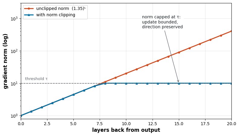
    Gradient norm exploding exponentially with depth and the same norm capped by gradient clipping

    Figure 1: Gradient norm flowing backward through a deep network: without control it grows geometrically layer by layer (note the log scale); gradient clipping caps the norm at a fixed threshold, keeping updates bounded regardless of depth.

    Mathematical Formulation:
    \frac{\partial L}{\partial z_l} = \frac{\partial L}{\partial z_n} \prod_{i=l}^{n-1} W_{i+1} \, f'(z_{i+1})
    \left\| \prod_i W_i \right\| \sim \prod_i \|W_i\|
    g \leftarrow g \cdot \min\!\left(1,\; \frac{\tau}{\|g\|}\right) \quad \text{(gradient clipping to threshold } \tau \text{)}

    Where:

    • z_l is the pre-activation of layer l; W_i and f'(z_i) are the per-layer weight and activation-derivative factors.
    • \|W_i\| is the operator (spectral) norm of the weight matrix; when the typical product exceeds 1, the gradient norm grows geometrically with depth.
    • g is the full gradient vector and \tau the clipping threshold: if \|g\| exceeds \tau, the gradient is rescaled down to norm \tau without changing its direction.

    Login to view more content
  • ML0024 Vanishing Gradient

    What are the typical reasons for vanishing gradient?

    Answer

    The vanishing gradient problem occurs when gradients shrink exponentially as they are backpropagated from the output layer toward the early layers of a deep network, so early layers receive almost no learning signal and train extremely slowly. The root cause is the chain rule: the gradient at an early layer is a product of many per-layer factors (weight matrices and activation derivatives), and if those factors are consistently smaller than 1 in magnitude, the product collapses toward zero as depth grows. The classic driver is saturating activation functions (sigmoid’s derivative peaks at only 0.25 and tanh’s at 1, and both are near zero for most of their input range), compounding with poor weight initialization that pushes pre-activations into the saturated tails. Recurrent networks suffer the same effect across time steps.

    (1) Saturating Activations: Sigmoid/tanh derivatives are small almost everywhere (sigmoid \sigma'(z) \leq 0.25); multiplying them across layers shrinks gradients exponentially.
    (2) Depth / Chain Rule: The gradient at layer 1 is a product of n per-layer factors; each factor below 1 makes the product vanish as n grows.
    (3) Poor Initialization: Too-large or too-small initial weights push activations into saturation, shrinking derivatives from the start.

    Gradient magnitude decaying exponentially with network depth on a log scale for sigmoid versus staying flat for ReLU

    Figure 1: Gradient magnitude at each layer during backpropagation (log scale): with sigmoid activations the signal decays roughly geometrically: after 20 layers the earliest layers receive gradients orders of magnitude smaller than the output layer.

    Mathematical Formulation:
    \frac{\partial L}{\partial z_l} = \frac{\partial L}{\partial z_{n}} \prod_{i=l}^{n-1} W_{i+1} \, f'(z_{i+1})
    \sigma(z) = \frac{1}{1 + e^{-z}}
    \sigma'(z) = \sigma(z)\big(1 - \sigma(z)\big) \leq 0.25

    Where:

    • z_l is the pre-activation of layer l, and n the total number of layers.
    • W_{i+1} is the weight matrix of layer i+1 and f'(\cdot) the activation derivative, the two per-layer factors in the chain product.
    • \sigma(z) is the sigmoid; its derivative peaks at 0.25 near z = 0 and approaches 0 in the saturated tails.
    Sigmoid curve with its derivative showing saturation regions where the derivative is near zero

    Figure 2: Why sigmoid kills gradients: outside the narrow active region around zero the derivative is essentially zero, so any neuron operating in the flat tails passes almost no gradient backward, and these small factors multiply down the chain.


    Login to view more content
  • ML0019 Imbalanced Data

    How to handle imbalanced data in Machine Learning?

    Answer

    Imbalanced data (where one class greatly outnumbers the other) skews models toward the majority class and must be handled deliberately. Five complementary techniques: resampling the dataset, by oversampling the minority class (e.g., SMOTE or ADASYN, which synthesize new minority points) or undersampling the majority class; data augmentation to create additional minority variants; class-weight adjustment, assigning a higher misclassification cost to the minority class during training; metric selection, evaluating with precision, recall, F1, or AUC-ROC rather than accuracy, which is misleading under imbalance; and algorithm selection, using specialized learners such as Balanced Random Forest or EasyEnsemble, or ensemble methods whose combined models are more robust to skewed classes.

    (1) Data-Level Fixes: Oversample the minority (SMOTE/ADASYN), undersample the majority, or augment minority samples.
    (2) Model-Level Fixes: Class weights in the loss, or imbalance-aware algorithms and ensembles.
    (3) Evaluation Fix: Never trust accuracy here; measure precision, recall, F1, or AUC.

    Imbalanced class distribution and SMOTE synthesizing minority samples

    Figure 1: Left: a 9:1 class imbalance. Right: SMOTE creates new minority points along the segments joining existing minority neighbors instead of duplicating them.

    Mathematical Formulation:
    x_{\mathrm{new}} = x_i + \lambda \, (x_{zi} - x_i), \quad \lambda \sim U(0,1)
    \mathcal{L} = \sum_{i} w_{y_i} \, \ell\big(f(x_i), y_i\big), \quad w_{c} \propto \frac{1}{n_c}

    Where:

    • x_{\mathrm{new}} is a synthetic minority sample created by SMOTE.
    • x_i is a minority sample and x_{zi} one of its nearest minority neighbors; \lambda is uniform in [0, 1], placing the new point somewhere on the connecting segment.
    • w_{y_i} is the per-sample weight from the class-weighting scheme; \ell is the per-sample loss and f the model.
    • n_c is the number of training samples of class c: the rarer the class, the higher its weight.

    Login to view more content