DL0059 Transposed Convolution

Written by

What is a transposed convolution (sometimes called deconvolution), and when is it used?

Answer

A transposed convolution is a learnable linear operator whose matrix is the transpose of the matrix representing a corresponding forward convolution. Operationally, each input value scatters a scaled kernel into an output grid, with stride controlling the spacing and overlapping contributions summed. It can increase spatial resolution, but it is not a mathematical inverse and does not recover information destroyed by downsampling. It is commonly used in semantic-segmentation decoders, generative models, learned reconstruction, and other architectures that map low-resolution features to higher-resolution outputs.

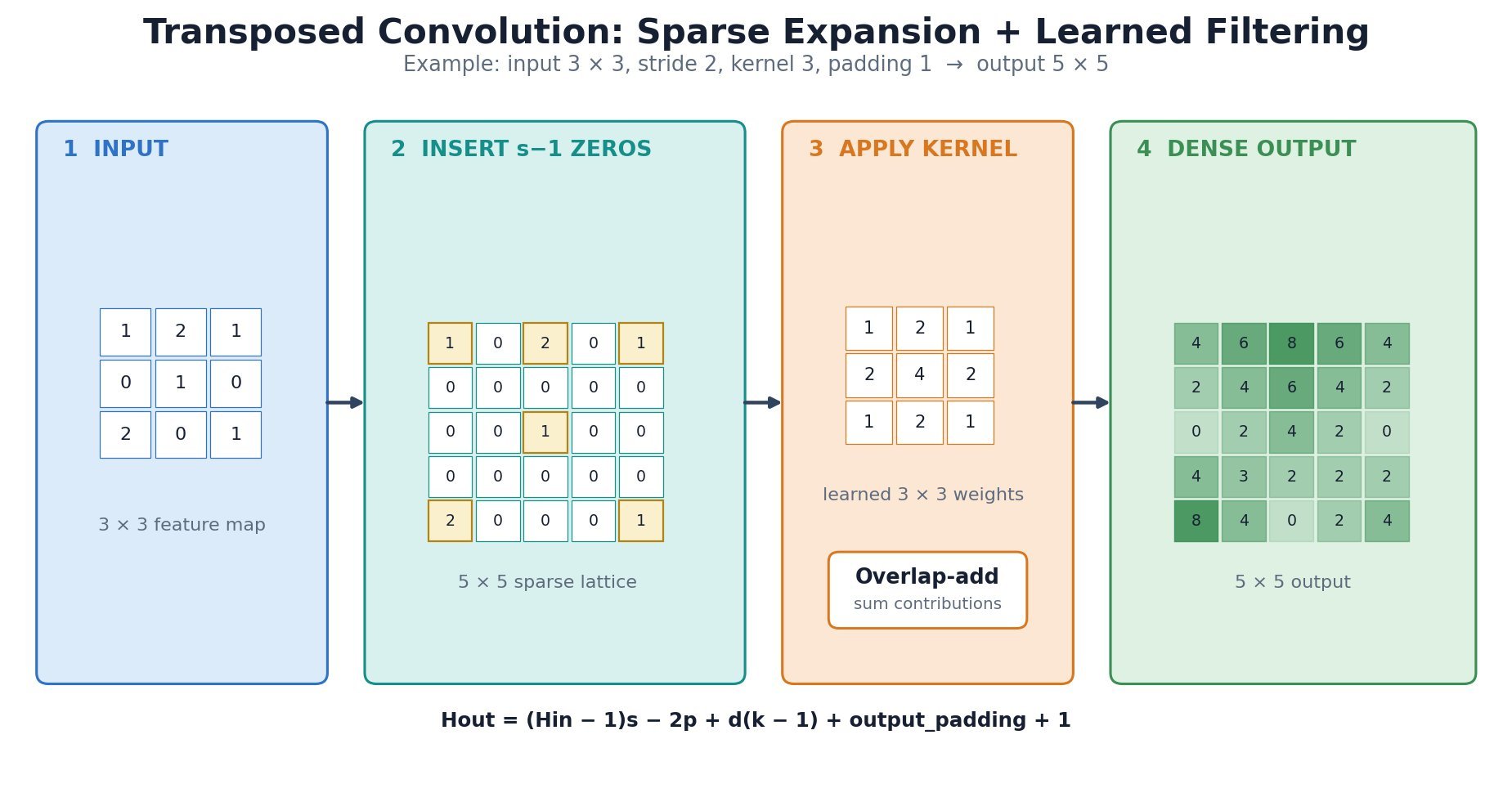
Transposed convolution shown as zero insertion, kernel application, and overlap summation.

Figure 1: A stride-2 transposed convolution decomposed into sparse expansion and learned filtering, including output-shape arithmetic.

(1) Learned Upsampling: Unlike fixed nearest-neighbor or bilinear interpolation, the layer learns how feature values contribute to surrounding output positions.
(2) Output Geometry: Kernel size, stride, padding, dilation, and output padding jointly determine the output shape; output padding resolves shape ambiguity but does not add zero-valued borders.
(3) Artifact Risk: Uneven overlap occurs when the kernel size is not divisible by stride and can produce checkerboard artifacts, especially in image generators.

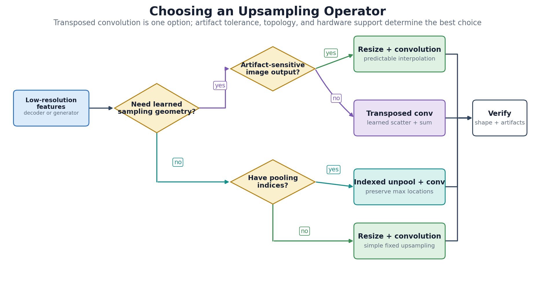
Upsampling-method decision flowchart comparing transposed convolution, resize-convolution, and unpooling.

Figure 2: Selection guide based on learned reconstruction, artifact sensitivity, pooling indices, and deployment constraints.

Mathematical Formulation:
$H_{out}=(H_{in}-1)s-2p+d(k-1)+p_{out}+1$

Where:

$H_{in}$ and $H_{out}$ are the input and output sizes along one spatial axis.
$s$ is stride, $p$ is padding, $d$ is dilation, and $k$ is kernel size.
$p_{out}$ is output padding used to choose among otherwise ambiguous valid output sizes; it does not append learned pixels.
The formula applies independently to width and, for 3D layers, depth by replacing $H$ with the corresponding axis size.