
What is depthwise separable convolution, and where is it commonly used?
Answer
Depthwise separable convolution factorizes a standard convolution into a depthwise spatial operation and a pointwise channel-mixing operation. The depthwise stage applies one  filter per input channel, so it learns spatial patterns independently; the
  pointwise stage combines those channel responses into new output channels. This factorization can reduce multiply-accumulates and parameters by almost the kernel area when channel counts are large. It is common in MobileNet, Xception, EfficientNet-style mobile blocks, and edge models where latency, power, and model size matter.
(1) Depthwise Stage: With depth multiplier one,  independent filters produce spatially filtered maps and do not mix channels.
(2) Pointwise Stage: A convolution applies a learned  channel transformation independently at every spatial position.
(3) Real Hardware: Lower arithmetic cost does not guarantee proportional speedup because memory traffic, kernel launch overhead, vectorization, and accelerator support can dominate.
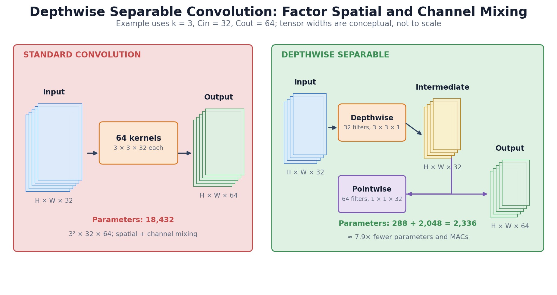
Figure 1: Tensor-level view of spatial filtering per channel followed by 1×1 channel mixing, with parameters and MACs.
Mathematical Formulation:


Where:
 and
and  count multiply-accumulates for standard and depthwise-separable convolution.
 and
and  are output height and width, and
  is the square spatial-kernel width.
 and
and  are input and output channel counts; the formula assumes depth multiplier
  .
.- For
 and large , the ratio approaches
  .
.
 and
and  count multiply-accumulates for standard and depthwise-separable convolution.
 and
and  are output height and width, and
  is the square spatial-kernel width.
 are input and output channel counts; the formula assumes depth multiplier
  .
. and large
  .
.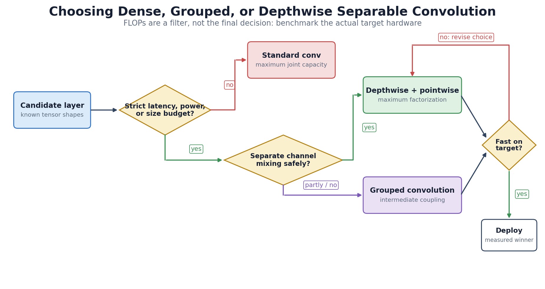
Figure 2: Architecture decision based on efficiency target, channel interaction, hardware kernels, and measured latency.
Leave a Reply