
When is distilling a large model into a small one a better strategy than serving the large model directly, for example behind a high-traffic assistant API?
Answer
Distillation wins when the recurring cost of inference, multiplied by sustained traffic, dominates the one-time cost of teacher labeling plus student training, and when the task distribution is narrow enough that the teacher’s surplus capability is never exercised. The decision is a break-even calculation: if the teacher costs $2.00 per 1k requests and an 8B student costs $0.25, and distillation costs $1,400 once (500k teacher-labeled prompts at $1,000 plus 200 GPU-hours at $400), the crossover is 800k requests, roughly 18 hours at 12 QPS. Two other conditions make distillation the only option rather than the cheapest one: a hard latency SLO that no batching strategy can meet with a 70B decoder, and a fixed memory envelope such as a phone NPU or a single 24 GB GPU, where quantization alone cannot close a 10x parameter gap. Serve the large model directly when traffic is low, when the input distribution is open-ended, or when the win is available more cheaply through quantization, speculative decoding, prompt caching, or a small-to-large cascade, since those preserve behavior and skip a new eval and re-qualification cycle. Distillation also carries a maintenance tax: every teacher upgrade reopens the labeling job, and the student inherits the teacher’s errors without the capacity to recover from them.
(1) Break-Even Volume: divide the one-time distillation cost by the per-request savings; below that volume, serving the teacher is strictly cheaper, and the payback period, not the compression ratio, is the number that decides the project.
(2) Latency Floor, Not Throughput: autoregressive decoding is memory-bandwidth bound and sequential, so per-token latency scales with parameter count and cannot be batched away; shrinking the model is one of the few levers that moves p99 rather than QPS per GPU.
(3) Task Breadth Decides Feasibility: on a stable, narrow task a student 8x smaller typically recovers 98-99% of teacher quality, while an open-ended assistant distribution loses many points because the teacher’s broad competence is exactly what is being compressed away.
(4) Hard Deployment Constraints: on-device, air-gapped, or offline targets impose a memory and power budget that no serving trick satisfies, so distillation becomes a requirement rather than an optimization.
(5) Cheaper Alternatives First: speculative decoding is distribution-preserving and needs no re-qualification, quantization is a one-line config change, and a router that sends easy traffic to a small model keeps the teacher available for the tail; distillation is the only lever that actually reduces the footprint, and it is the most expensive to maintain.
Mathematical Formulation:


Where:
 is the break-even request volume, the point at which cumulative distilled-serving cost equals cumulative teacher-serving cost.
- and are the marginal serving costs per request for the large teacher and the small student; the difference must be positive for distillation to ever pay back.
- is the one-time cost, composed of teacher inference over unlabeled prompts plus student training ; engineering and eval time belong here too and usually exceed the compute.
- is the student objective, mixing hard-label cross-entropy with the distillation term under mixing weight .
- is the softmax temperature applied to both teacher and student logits, and the factor rescales the gradient so stays meaningful as changes; and are the tempered teacher and student distributions.
- Required condition for the whole strategy: the student must also satisfy the latency and memory constraints, and , which no amount of traffic volume can buy.
 is the break-even request volume, the point at which cumulative distilled-serving cost equals cumulative teacher-serving cost.
 and
 are the marginal serving costs per request for the large teacher and the small student; the difference
 must be positive for distillation to ever pay back.
 is the one-time cost, composed of teacher inference over
 unlabeled prompts plus student training
 ; engineering and eval time belong here too and usually exceed the compute.
 is the student objective, mixing hard-label cross-entropy
 with the distillation term
 under mixing weight
 .
 is the softmax temperature applied to both teacher and student logits, and the
 factor rescales the gradient so
 stays meaningful as
 and
 are the tempered teacher and student distributions.
 and
 , which no amount of traffic volume can buy.
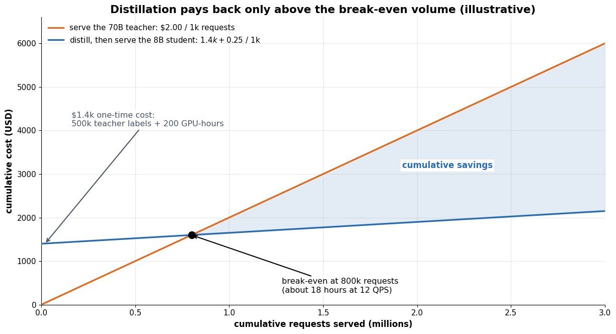
Figure 1: Illustrative cost curves: the distilled path carries a $1.4k fixed intercept but an eight-times shallower slope, so the break-even sits at 800k requests and every request after that is pure savings.
The break-even math is only valid if the student actually holds quality on the traffic you will receive, and that depends far more on task breadth than on the compression ratio. A single-intent classifier, a fixed extraction schema, or one product domain compresses well because the teacher’s decision boundary in that slice is simple and you can generate unlimited soft targets for it; an open-ended assistant does not, because the surplus capacity is the product. When breadth is the problem, a cascade is usually the better answer than a bigger student: route every request to the distilled model, escalate the tail flagged by a confidence or verifier signal to the teacher, and you capture most of the cost win while keeping the quality ceiling. Whatever you choose, budget for the maintenance tax, since a teacher upgrade invalidates the student, drifting inputs silently move outside the distilled distribution, and you now own two eval suites instead of one.

Figure 2: Illustrative quality retention: on a narrow task a 1B student already clears a 98% floor, while the same student on open-ended traffic gives up roughly 27 points, which is why breadth, not the compression factor, gates the decision.
| Property | Distill to a small student | Serve large + quantization | Serve large + speculative decoding |
|---|---|---|---|
| Memory footprint | 8-20x smaller, can drop from 8 GPUs to 1 or to a phone | 2-4x smaller weights, KV cache mostly unchanged | Slightly larger, the drafter is an extra resident model |
| Quality guarantee | None, must be re-measured per task; tail regressions are common | Small measurable drift, worse at 4-bit and on long context | Distribution-preserving, output matches the teacher exactly |
| Typical latency gain | 4-6x on per-token latency, the largest available lever | 1.5-2.5x, bounded by bandwidth saved on weights | 2-3x at low batch, degrades as batch size grows |
| One-time cost | Label generation, training runs, a new eval harness | Calibration pass plus a quality spot-check | Serving-stack work, no retraining of the target model |
| Cost when the teacher is upgraded | Full re-distillation and re-qualification | Re-run calibration only | Swap the target, optionally refresh the drafter |
| Wins when | High sustained traffic, narrow task, or a fixed device budget | You need a fast, low-risk cost cut on broad traffic | Latency matters, batches are small, and quality cannot move |
Leave a Reply