Tag: Basics

  • ML0046 Forward Propagation

    Please explain the process of Forward Propagation.

    Answer

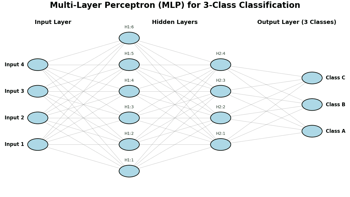
    Forward propagation is when a neural network takes an input and generates a prediction. It involves systematically passing the input data through each layer of the network. A weighted sum of the inputs from the previous layer is calculated at each neuron, and then a nonlinear activation function is applied. This process is repeated layer by layer until the data reaches the output layer, where the final prediction is generated.

    Here is the process of Forward Propagation:
    (1) Input Layer: The network receives the raw input data.
    (2) Layer-wise Processing:
    Linear Combination: Each neuron calculates a weighted sum of its inputs and adds a bias.
    Non-linear Activation: The resulting value is passed through an activation function (e.g., ReLU, sigmoid, tanh) to introduce non-linearity.
    (3) Propagation Through Layers: The output from one layer becomes the input for the next layer, progressing through all hidden layers.
    (4) Output Generation: The final layer applies a function (like softmax for classification or a linear function for regression) to produce the network’s prediction.


    Login to view more content

  • ML0045 Multi-Layer Perceptron

    What is a Multi-Layer Perceptron (MLP)? How does it overcome Perceptron limitations?

    Answer

    A Multi-Layer Perceptron (MLP) is a feedforward neural network with one or more hidden layers between the input and output layers. Hidden layers in MLP use non-linear activation functions (like ReLU, sigmoid, or tanh) to model complex relationships. MLP can be used for classification, regression, and function approximation. MLP is trained using backpropagation, which adjusts the weights to minimize errors.

    Overcoming Limitations:
    (1) Learn non-linear: Unlike a single-layer perceptron that can only solve linearly separable problems, an MLP can learn non-linear decision boundaries, handling problems such as the XOR problem.
    (2) Universal Approximation: With enough neurons and layers, an MLP can approximate any continuous function, making it a powerful model for various applications.

    The plot below illustrates an example of a Multi-Layer Perceptron (MLP) applied to a classification problem.


    Login to view more content
  • ML0044 Perceptron

    Describe the Perceptron and its limitations.

    Answer

    The perceptron is a simple linear classifier that computes a weighted sum of input features, adds a bias, and applies a step function to produce a binary decision. The perceptron works well only for data sets that are linearly separable, where a straight line (or hyperplane in higher dimensions) can separate the classes.

    The perception output can be calculated by
     y = f(w^T x + b)
    Where:
     y is the predicted output (0 or 1)
     w is the weight vector
     x is the input vector
     b is the bias term
     f(\cdot) is the activation function (typically a step function)

    Below shows a perceptron diagram.

    Limitations for using perception:
    (1) Linearly Separable Data Only: Cannot solve problems like XOR, which are not linearly separable.
    (2) Single-Layer Only: Cannot model complex or non-linear patterns.
    (3) No Probabilistic Output: Outputs only binary values, not confidence or probabilities.


    Login to view more content
  • DL0015 Cold Start

    What is a “cold start” problem in deep learning?

    Answer

    The cold start problem is the difficulty of making reliable predictions for new entities (such as users, items, or contexts) lacking historical data.
    Many deep learning models, especially in recommendation systems, rely on abundant past data to learn meaningful patterns. When a new user or item is introduced, the model struggles because it doesn’t have enough information to produce accurate predictions.

    Mitigation Strategies for the Cold Start Problem:
    (1) Transfer Learning / Pretrained Models: Use embeddings or models pre-trained on similar tasks to provide a starting point.
    (2) Hybrid Recommendation Models: Combine collaborative filtering (CF) and content-based methods.
    (3) Active Learning / User Onboarding: Actively gather more data for new entities through user interactions.


    Login to view more content
  • ML0042 Early Stopping

    What is Early Stopping? How is it implemented?

    Answer

    Early Stopping is a regularization technique used to halt training when a model’s performance on a validation set stops improving, thus avoiding overfitting. It monitors metrics like validation loss or validation accuracy and stops after a defined number of stagnant epochs (patience). This ensures efficient training and better generalization.

    Implementation:
    Split data into training and validation sets.
    After each epoch, evaluate on the validation set.
    If performance improves, save the model and reset the patience counter.
    If no improvement, counter add one; if the counter reaches the patience epochs, stop training.
    Restore best weights after stopping, load the model weights from the epoch that yielded the best validation performance.

    Below is one example loss plot when using early stop.


    Login to view more content
  • ML0041 Concept of NN

    Please explain the concept of a Neural Network.

    Answer

    A neural network (NN) is a machine learning model composed of layers of interconnected neurons. It learns patterns in data by adjusting weights through training, enabling it to perform tasks like classification, regression, and more.

    (1) Inspired by Biology: Neural networks are computer systems modeled after the human brain’s network of neurons.
    (2) Layered Structure: Neural networks consist of an input layer, one or more hidden layers, and an output layer.
    (3) Neurons and Activation: Each neuron performs a weighted sum of its inputs, adds a bias, and applies an activation function to produce an output. Weights and Biases are learnable parameters adjusted during training. Activation Functions can introduce non-linearity (e.g., ReLU, Sigmoid).
    (4) Learning Process: Neural networks learn by adjusting the weights and biases through training algorithms such as backpropagation, minimizing errors between predictions and actual results.
    (5) Versatility in Applications: Neural networks can identify complex patterns, making them suitable for tasks like image recognition, natural language processing, and data classification.

    Below shows an example of an NN.


    Login to view more content
  • DL0014 Mixed Precision Training

    Can you explain the primary benefits of using mixed precision training in deep learning?

    Answer

    Mixed precision training accelerates deep learning by using both FP32 and FP16 operations, which reduces memory and computational requirements while maintaining model accuracy, resulting in faster and more efficient training.

    (1) Faster Training: Uses lower-precision (e.g., FP16) operations on supported hardware (like GPUs/TPUs), which are faster than FP32.
    (2) Reduced Memory Usage: Lower-bit representations decrease memory footprint, allowing larger batch sizes or models.
    (3) Higher Throughput: More computations per second due to reduced precision, which can speed up training time.
    (4) Supports Large Models: Enables training of models that wouldn’t fit in memory with full precision.
    (5) Maintains Accuracy: With proper scaling (e.g., loss scaling), training stability and final model accuracy can typically be preserved.


    Login to view more content
  • ML0040 Bias and Variance

    Can you explain the bias-variance tradeoff?

    Answer

    Bias:
    Error due to overly simplified assumptions in the model.
    High bias may lead to underfitting, where the model misses key patterns in the data.

    Variance:
    Error due to high sensitivity to variations in the training data.
    High variance may result in overfitting, where the model captures noise and underlying patterns.

    Bias-Variance Tradeoff:
    Increasing model complexity typically decreases bias but increases variance, while a simpler model increases bias but decreases variance.
    The goal is to balance both to minimize the total error on unseen data.

    The bias-variance tradeoff illustrates that there’s a delicate balance to strike when building a machine learning model. A simpler model tends to have high bias and low variance, underfitting the data. A more complex model tends to have low bias and high variance, overfitting the data. The goal is to find the right level of model complexity to minimize the total prediction error, which is the sum of squared bias, variance, and irreducible error.

    The example below shows scenarios of high bias (underfitting), high variance (overfitting), and a good balance.


    Login to view more content

  • ML0039 Distributed Training

    What are the two main distributed training approaches for machine learning?

    Answer

    The two main distributed training approaches for machine learning are Data Parallelism and Model Parallelism.

    Data Parallelism: In this approach, the training dataset is divided and distributed among multiple computing devices, with each device holding a complete copy of the machine learning model. Each device then trains its model on its assigned subset of the data in parallel. After each training step, the updates (gradients or new parameters) from all devices are aggregated and synchronized to maintain a consistent model across the system. This method is highly effective for scaling training when the dataset is large and the model can fit within a single device’s memory.

    Model Parallelism: This approach is used when the machine learning model itself is too large to fit into the memory of a single computing device. In model parallelism, different parts of the model (e.g., specific layers of a neural network) are distributed across multiple devices. Data typically flows sequentially through these distributed model parts. This necessitates more complex communication between devices as intermediate computations and activations must be passed along. Model parallelism is crucial for training extremely large models that would otherwise be computationally intractable on a single machine.


    Login to view more content
  • ML0035 Model Comparison

    How to compare different machine learning models?

    Answer

    Compare machine learning models by defining clear objectives and metrics, using consistent data splits, training and tuning each model, and evaluating them through robust metrics and statistical tests. Finally, consider trade-offs like model complexity and interpretability to make an informed choice.
    (1) Choose Relevant Metrics: Select evaluation metrics that align with your task (e.g., accuracy or F1 for classification)
    Below shows an example using ROC curves for model comparison.

    (2) Use Consistent Data Splits: Evaluate all models on the same train/validation/test splits—or identical cross-validation folds—to ensure fairness
    (3) Apply Cross-Validation: Employ k-fold or nested cross-validation to reduce variance in performance estimates, especially with limited data
    (4) Control Randomness: Run each model multiple times with different random seeds (data shuffles, weight initializations) and average the results to gauge stability
    (5) Perform Statistical Tests: Use paired tests to determine if observed differences are statistically significant
    (6) Measure Efficiency: Record training time, inference latency, and resource usage (CPU/GPU and memory) to assess practical deployability
    (7) Evaluate Robustness & Interpretability: Test models under data perturbations or adversarial noise, and compare explainability


    Login to view more content