Interview for Machine Learning

Tag: Transformer

DL0044 Multi-Query Attention
What is Multi-Query Attention in transformer models?
Answer
Multi-Query Attention (MQA) optimizes the standard Multi-Head Attention (MHA) in transformers by using multiple query heads while sharing a single key-value projection across them. This design maintains similar computational expressiveness to MHA but significantly reduces memory usage during inference, especially in KV caching for autoregressive tasks, making it ideal for scaling large models. It trades minor potential quality for efficiency.
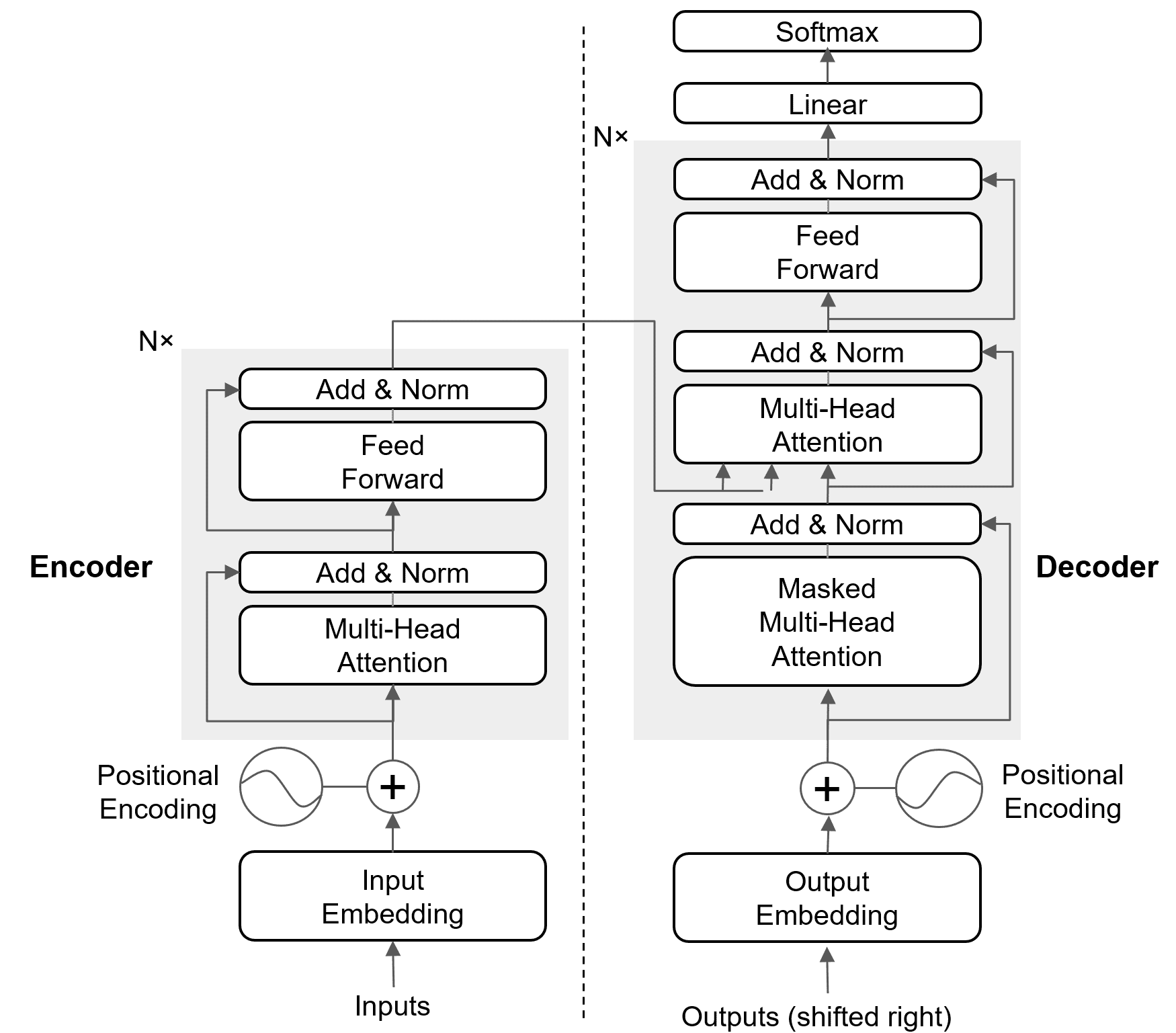
Comparison to Multi-Head Attention (MHA): In standard MHA, each attention head has independent projections for queries (Q), keys (K), and values (V). In MQA, only Q is projected into multiple heads, while K and V use a single projection shared across all query heads, as shown in the figure below.
Efficiency Benefits: Reduces memory footprint during inference, particularly with KV caching, as the cache stores only one set of K and V vectors instead of one per head, lowering memory complexity from O(n * h * d) to O(n * d), where n is sequence length, h is number of heads, and d is head dimension.
The core attention operation for a single head in MQA can be represented by the following equation:
$\mbox{Attention}(Q_i, K_{shared}, V_{shared}) = \mbox{Softmax}(\frac{Q_i K_{shared}^T}{\sqrt{d_k}}) V_{shared}$
Where:
$Q_i$ represents the query vector for the ith attention head.
$K_{shared}$ and $V_{shared}$ represent the single, shared key and value vectors used by all heads.
$d_k$ is the dimension of the key vectors.
Login to view more content
September 14, 2025
DL0043 KV Cache
What is KV Cache in transformers, and why is it useful during inference?
Answer
The KV Cache in transformers optimizes inference by storing and reusing key and value vectors from the attention mechanism, avoiding redundant computations for previous tokens in a sequence. This is particularly useful in autoregressive models, where each new token requires attention over all prior tokens. By caching K and V vectors, the model only computes the query for the new token and retrieves cached K and V for earlier tokens, improving speed at the cost of higher memory usage.
The attention mechanism, optimized by KV Cache, is:
$\mathrm{Attention}(Q_t, K_{1:t}, V_{1:t}) = \mathrm{Softmax}\left(\frac{Q_t K_{1:t}^\top}{\sqrt{d_k}}\right) V_{1:t}$
Where:
$Q_t$ = query of the current token t.
$K_{1:t}, V_{1:t}$ = cached keys and values for all tokens up to t.
$d_k$ = key dimension.
The figure below explains the KV cache in autoregressive transformers.
Login to view more content
September 14, 2025
DL0042 Attention Computation
Please break down the computational cost of attention.
Answer
Here is the breakdown of the computational cost of attention:
$\mathcal{O}(n^2 \cdot d + n \cdot d^2)$
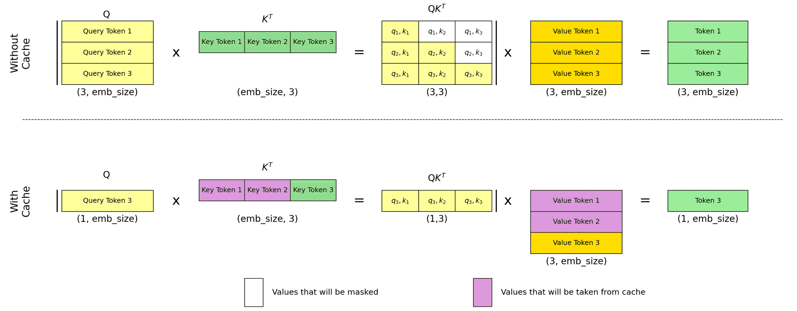
Input dimensions: Sequence length = $n$ , hidden dimension = $d$ , number of heads = $h$ .
(1) Linear projections (Q, K, V):
Each input $X \in \mathbb{R}^{n \times d}$ is projected into queries, keys, and values.
Cost: $\mathcal{O}(n \cdot d^2)$ (for all 3 matrices).
(2) Attention score computation (QKᵀ):
Queries: $Q \in \mathbb{R}^{n \times d_k}$
Keys: $K \in \mathbb{R}^{n \times d_k}$
Score matrix:
$S = QK^\top \in \mathbb{R}^{n \times n}$
Cost: $\mathcal{O}(n^2 \cdot d_k)$
(3) Softmax normalization:
For each row of the score matrix:
$\mbox{Softmax}(s_i) = \frac{e^{s_i}}{\sum_{j=1}^n e^{s_j}}$
Where:
$s_i$ = raw score for position $i$
$n$ = total sequence length
Cost: $\mathcal{O}(n^2)$
(4) Weighted sum with values (AV):
Attention weights $A \in \mathbb{R}^{n \times n}$ applied to values $V \in \mathbb{R}^{n \times d_v}$ :
$O = AV$
Cost: $\mathcal{O}(n^2 \cdot d_v)$
(5) Output projection:
Final linear layer to mix heads back to $d$ .
Cost: $\mathcal{O}(n \cdot d^2)$
Total Complexity:
Putting it all together:
$\mathcal{O}(n \cdot d^2) + \mathcal{O}(n^2 \cdot d_k) + \mathcal{O}(n^2 \cdot d_v)$
Since $d_k, d_v \approx d/h$ , the dominant term is:
$\mathcal{O}(n^2 \cdot d + n \cdot d^2)$
Overall, the cost of Multi-Head Attention (MHA)is in the same order as single-head, because per-head dims scale as $d/h$ .
Login to view more content
September 6, 2025
DL0041 Hierarchical Attention
Could you explain the concept of hierarchical attention in transformer architectures?
Answer
Hierarchical Attention in Transformers applies self-attention at multiple levels of granularity (e.g., words to sentences to documents). Instead of one flat attention over all tokens, it computes local attention within segments and then global attention across segments, leading to efficiency gains, better structure modeling, and interpretable focus at each level.
Motivation: Transformers normally apply flat self-attention over all tokens. For long structured inputs (documents, videos, graphs), this is inefficient and loses hierarchical structure.
Hierarchical Attention Idea:
(1) Local level (fine-grained): Compute attention within smaller segments (e.g., words within a sentence, frames within a shot).
(2) Global level (coarse-grained): Aggregate segment representations, then apply attention across segments (e.g., sentences within a document, shots within a video).
This mirrors natural data hierarchies and reduces quadratic cost.
The figure below shows Hierarchical Attention used in the document classification use case.
Login to view more content
September 1, 2025
DL0040 Attention Mask
What is the role of masking in attention?
Answer
Masking is a critical technique in transformer attention mechanisms that controls which parts of the input sequence the model is allowed to focus on.
(1) Leakage prevention: Blocks access to future tokens in autoregressive decoding to preserve causality.
(2) Padding handling: Excludes pad positions so they don’t absorb probability mass or distort context.
(3) Structured constraint: Enforces task rules (e.g., graph neighborhoods, spans, or blocked regions).
Core equation with mask:
$\text{Attn}(Q,K,V,M)=\text{Softmax}\left(\frac{QK^\top}{\sqrt{d_k}}+M\right)V$
Where:
$Q$ query matrix.
$K$ key matrix.
$V$ value matrix.
$d_k$ key dimensionality (for scaling).
$M$ mask matrix with 0 for allowed positions and large negative values (e.g., −∞) for disallowed positions.
The figure below shows three side-by-side heatmaps: a padding mask that disallows attending to padding tokens, a causal mask that enforces autoregressive decoding, and a structured mask that enforces local neighborhood constraint.
Login to view more content
August 31, 2025
DL0039 Transformer Weight Tying
Explain weight sharing in Transformers.
Answer
Weight sharing in Transformers mainly refers to tying the input embedding matrix with the output projection matrix for softmax prediction, saving parameters, and improving consistency. In some models (like ALBERT), it also extends to sharing weights across Transformer layers for further parameter efficiency.
(1) Input–Output Embedding Tying:
The same embedding matrix is used for both input token embeddings and the output softmax projection.
Reduces parameters and enforces consistency between input and output spaces.
$\mbox{Softmax}(z_i) = \frac{e^{z_i}}{\sum_{j=1}^{K} e^{z_j}}$
Where:
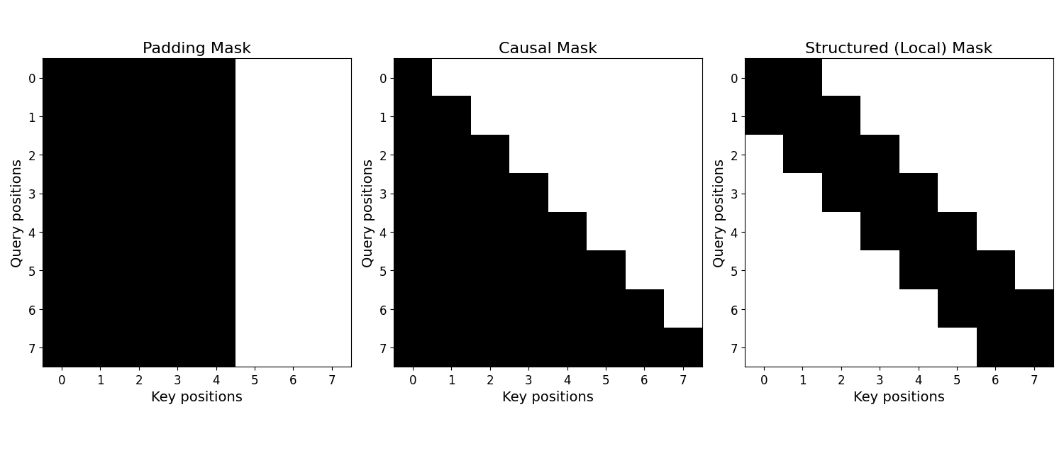
$z_i = (E h)_i$ is the logit for token $i$ , computed using the embedding matrix $E \in \mathbb{R}^{K \times d}$ .
$h \in \mathbb{R}^{d}$ is the hidden representation from the Transformer.
$K$ is the vocabulary size.
Weights tying are shown in the figure below.
(2) Layer Weight Sharing (e.g., ALBERT [1]):
Instead of unique weights per layer, parameters are reused across all Transformer blocks.
Cuts model size dramatically while keeping depth.
References:
[1] Lan, Zhenzhong, et al. “Albert: A lite bert for self-supervised learning of language representations.” arXiv preprint arXiv:1909.11942 (2019).
Login to view more content
August 28, 2025
DL0038 Transformer Activation
Which activation functions do transformer models use?
Answer
Transformers mainly use GELU/ReLU in the feed-forward layers to introduce non-linearity and Softmax in attention to produce normalized attention weights. GELU is preferred for smoother gradient flow and better performance.
(1) Feed-Forward Network (FFN):
Uses ReLU or GELU as the non-linear activation.
GELU is more common in modern Transformers (like BERT, GPT).
Equation for GELU:
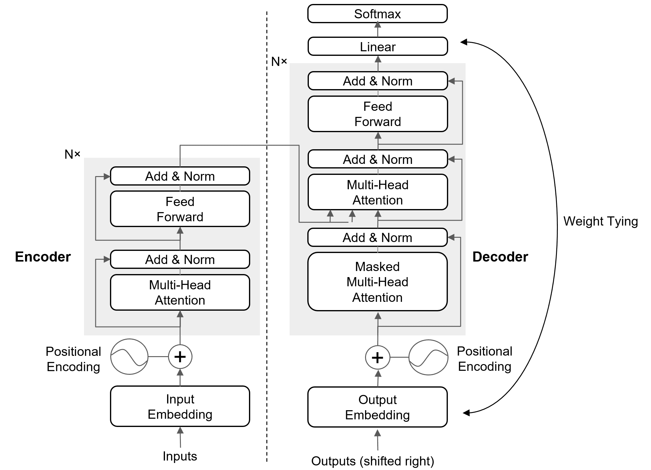
$\mbox{GELU}(x) = x \cdot \Phi(x) = x \cdot \frac{1}{2}\left[1 + \mbox{erf}\left(\frac{x}{\sqrt{2}}\right)\right]$
Where:
$x$ is the input,
$\Phi(x)$ is the Cumulative Distribution Function (CDF) of the standard Gaussian.
The figure below demonstrates the difference between ReLU and GELU.
(2) Attention Output:
Uses Softmax to convert attention scores into probabilities.
Equation for Softmax:
$\mbox{Softmax}(z_i) = \frac{e^{z_i}}{\sum_{j=1}^{K} e^{z_j}}$
Where:
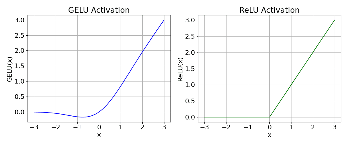
$z_i$ represents the raw attention score for the i-th token,
$K$ is the total number of tokens considered in attention.
Login to view more content
August 26, 2025
DL0037 Transformer Architecture III
Why do Transformers use a dot product, rather than addition, to compute attention scores?
Answer
Dot product attention is a fast and naturally aligned similarity measure; with scaling, it remains numerically stable and highly parallelizable, which is why Transformers prefer it over addition.
(1) Dot product captures similarity: The dot product between query $q$ and key $k$ grows larger when they point in similar directions, making it a natural similarity measure.
The scores are normalized with Softmax and have probabilistic interpretations:
$\alpha_i = \frac{e^{q \cdot k_i}}{\sum_{j=1}^K e^{q \cdot k_j}}$
Where:
$q \cdot k_i$ is the dot product similarity between query and key.
The figure below illustrates the dot product for measuring similarity.

(2) Efficient computation: Dot products can be computed in parallel as a matrix multiplication $QK^\top$ , which is hardware-friendly.
Login to view more content
August 26, 2025
DL0036 Transformer Architecture II
What are the main differences between the encoder and decoder in a Transformer?
Answer
The encoder focuses on encoding input into rich representations via bidirectional self-attention, while the decoder leverages these for output generation through masked self-attention and cross-attention, ensuring autoregressive and context-aware predictions.
(1) Self‑Attention:
Encoder: Unmasked, attends to all positions in the input sequence.
Decoder: Masked, attends only to past positions to maintain causal order.
(2) Cross‑Attention:
Encoder: None.
Decoder: Present — attends to encoder outputs for context.
(3) Masking:
Encoder: No masking needed.
Decoder: Causal mask prevents looking ahead.
(4) Positional Encoding:
Encoder: Added to source embeddings.
Decoder: Added to target embeddings (shifted right during training).
(5) Function:
Encoder: Encodes the full source sequence into contextual representations.
Decoder: Generates the target sequence one token at a time using its own history and encoder context.
The figure below shows the encoder and the decoder in the Transformer.
Login to view more content
August 17, 2025
DL0035 Transformer Architecture
Describe the original Transformer encoder–decoder architecture.
Answer
The original Transformer model has an encoder-decoder architecture. The encoder processes the input sequence (e.g., a sentence) to create a contextual representation for each word. The decoder then uses this representation to generate the output sequence (e.g., the translated sentence), one word at a time. This entire process relies on attention mechanisms instead of recurrence.
Overall: Sequence-to-sequence encoder–decoder model with 6 encoder layers and 6 decoder layers [1].
Encoder layer:
(1) Multi-Head Self-Attention (all tokens attend to each other).
(2) Position-wise Feed-Forward Network (two linear layers + ReLU).
(3) Residual connection + LayerNorm after each sublayer.
Decoder layer:
(1) Masked Multi-Head Self-Attention (prevents seeing future tokens).
(2) Cross-Attention (queries from decoder, keys/values from encoder output).
(3) Position-wise Feed-Forward Network.
(4) Residual connection + LayerNorm after each sublayer.
Input representation: Inputs are represented as token embeddings summed with positional encodings to preserve sequence order, as the attention mechanism is permutation-invariant.
Output: The final decoder output passes through a linear projection layer, followed by softmax to produce probabilities over the target vocabulary for next-token prediction.
The figure below shows the architecture of the Transformer.

References:
[1] Vaswani, Ashish, et al. “Attention is all you need.” Advances in neural information processing systems 30 (2017).
Login to view more content
August 14, 2025