Author: admin

DL0110 VLM Image-Text Token Alignment

How do you align image tokens with text tokens in a vision-language model, for example in a system like LLaVA or Qwen2-VL?

Answer

Alignment is not one operation but three that have to agree: a representation map, a sequence layout, and a training curriculum. The dominant recipe runs a frozen contrastive vision encoder over the image, then a small trainable connector projects every patch embedding into the LLM’s token embedding space so the image becomes a block of ordinary tokens occupying real sequence positions. A CLIP ViT-L/14 at $336 \times 336$ produces $24 \times 24 = 576$ patch embeddings of width 1024, and a two-layer MLP maps them to the LLM width (4096 for a 7B decoder); the tokenizer’s single image placeholder is expanded in place into those 576 vectors. From that point alignment is learned by plain next-token prediction: text tokens read image positions through the same causal self-attention, and the gradient of the caption loss is what teaches the connector which visual direction means “a red bus”. The competing topology keeps images out of the sequence entirely and injects them through gated cross-attention layers inserted into a frozen LLM, as in Flamingo and Llama 3.2 Vision, trading sequence length for extra parameters.

(1) Shared Embedding Space: the connector’s only job is to land visual features in the same $d_{\text{model}}$ -dimensional space the token embedding table lives in, which is why an MLP with roughly 20M parameters is enough.
(2) Placeholder Expansion: the prompt carries one image placeholder id, and at embedding time that row is replaced by the $N$ projected vectors, so nothing downstream of the embedding layer knows the difference.
(3) Positional Alignment: patches are flattened row-major, so a purely 1D RoPE makes a vertical neighbor 24 positions away; 2D or multimodal RoPE restores height and width structure explicitly.
(4) Two Injection Topologies: prefix tokens with full self-attention are simple and preserve fine detail; gated cross-attention keeps the text stream’s length untouched and protects text-only ability.
(5) Staged Curriculum: stage 1 tunes only the connector on image-caption pairs with a frozen encoder and LLM, then stage 2 unfreezes the LLM on instruction data.
(6) Token Budget Is The Real Constraint: prefill attention is $O(L^2)$ in total sequence length, so pixel unshuffle, learned query resamplers, and tiling policies exist purely to control $N$ .

Pipeline diagram: a 336 by 336 image is encoded by a frozen ViT-L/14 into 576 patch features of width 1024, an MLP connector projects them to 4096 dimensions, and the resulting image tokens are spliced into the LLM token sequence between text embeddings before a causal decoder stack

Figure 1: The connector is the only trainable component in stage 1; after projection the 576 image tokens are indistinguishable from text embeddings to the decoder, which fuses both streams in a single causal self-attention stack.

Two details decide whether the alignment survives at scale. The first is resolution: a fixed $336 \times 336$ view destroys the small text and thin structures that document and chart questions depend on, so production models either tile the image into crops plus a downscaled thumbnail (AnyRes) or feed native resolution with a variable token count. The second is cost: because prefill attention grows quadratically, an AnyRes scheme with four crops plus a thumbnail spends 2,880 image tokens and roughly 25x the attention work of one 576-token view, before a single text token is generated. Compression is the usual answer, either a $2 \times 2$ pixel unshuffle that folds four patches into one channel-concatenated token or a query-based resampler that squeezes any number of patches into 32 or 64 learned slots. Both save compute by throwing away exactly the spatial precision that grounding and OCR need, which is why token budget, not connector architecture, is where most VLM design arguments actually land.

Mathematical Formulation:
$Z_v = g_{\phi}(x_{\text{img}})$
$H_v = W_2\,\sigma(W_1 Z_v)$
$N = \frac{H W}{P^2 r^2}$
$N = \frac{336 \cdot 336}{14^2 \cdot 1} = 576$
$E = [\, e(t_{1:k}),\; H_v,\; e(t_{k+1:m}) \,]$
$\mathcal{L} = -\sum_{i} \log p_{\theta}(t_i \mid t_{1:i-1}, H_v)$

Where:

$x_{\text{img}}$ is the image and $g_{\phi}$ the frozen vision encoder, giving patch features $Z_v \in \mathbb{R}^{N \times d_v}$ with $d_v = 1024$ for ViT-L.
$W_1, W_2$ and the nonlinearity $\sigma$ form the MLP connector, producing $H_v \in \mathbb{R}^{N \times d_{\text{model}}}$ in the LLM embedding space.
$H, W$ are image height and width, $P$ the patch size, and $r$ the pixel-unshuffle factor ( $r = 1$ means no merging, $r = 2$ cuts tokens 4x).
$e(\cdot)$ is the text embedding lookup, $t_{1:m}$ the prompt and response tokens, and $k$ the position of the image placeholder that $H_v$ replaces.
$E$ is the assembled input of length $L = m + N - 1$ , and $\mathcal{L}$ is the autoregressive loss masked to response tokens only, so no loss is computed on image positions.
Required initial condition: $g_{\phi}$ must already be language-aligned (CLIP or SigLIP pretraining), otherwise stage 1 has to learn the semantics as well as the projection.

Bar chart of image token counts and relative prefill attention cost for four vision-language configurations: 576 tokens at 1x, 1280 tokens at 4.9x, 1536 tokens at 7.1x, and 2880 tokens at 25x

Figure 2: Higher-resolution alignment policies buy detail with sequence length, and since prefill attention is $O(L^2)$ , moving from a single 576-token view to a five-crop AnyRes layout costs about 25x the attention work per prompt.

Property	MLP connector (prefix tokens)	Query resampler (Q-Former, Perceiver)	Gated cross-attention
Where fusion happens	In the input sequence, before layer 1	In the connector, then in the input sequence	Inside the decoder, at interleaved new layers
Tokens added to the LLM sequence	One per patch, 576 to 2,880 typical	Fixed, 32 to 64 regardless of resolution	Zero
New parameters	Smallest, roughly 20M for a 7B model	Moderate, a small transformer plus queries	Largest, extra attention plus tanh gates in the decoder
Prefill and KV-cache cost	Grows quadratically with token count	Nearly flat in image resolution	Linear in image features, no text-side growth
Typical failure mode	Latency and context blowup on multi-image or video prompts	Information bottleneck: weak OCR, dense counting, fine grounding	Harder to train, weaker at precise pixel-level reference
Text-only ability	Can regress once the LLM is unfrozen	Same risk if the LLM is tuned	Preserved by construction with a frozen LLM and zero-init gates

August 17, 2026

DL0109 Mixture-of-Experts MoE Routing

Explain mixture-of-experts (MoE) and compare Sparse Mixture-of-Experts (MoE) routing strategies, as used in models like Mixtral and DeepSeek-V3.

Answer

A sparse mixture-of-experts layer replaces one feed-forward block with $N$ parallel feed-forward blocks (the experts) plus a tiny linear router, and sends each token to only $k \ll N$ of them. This is conditional computation: parameter count grows with $N$ while the FLOPs per token grow only with $k$ , so Mixtral 8x7B holds 46.7B parameters but activates about 12.9B per token, and DeepSeek-V3 holds 671B while activating 37B. The interesting engineering is not the experts, which are ordinary MLPs, but the routing strategy, because a learned router is free to collapse onto a few favorite experts and then most of the capacity you paid for is never trained. The dominant strategy is token-choice top-k: every token picks its own $k$ experts, each expert has a fixed buffer set by a capacity factor, and tokens that arrive at a full expert are dropped through the residual connection. The main alternatives invert or remove that choice: expert-choice routing lets each expert select its top tokens (perfect load balance, but some tokens get no expert), hash layers assign tokens deterministically with no learned router at all, and BASE layers solve a global linear assignment per batch. The trade-off axis is always the same, namely how much balance you buy and what you pay for it in dropped tokens, extra loss terms, batch dependence, and all-to-all communication.

(1) Parameters Decouple From FLOPs: with $N=8, k=2$ a token touches 25% of the expert weights, so quality scales with total parameters while latency scales with active parameters.
(2) The Router Is One Matrix: a single $d \times N$ projection followed by top-k selection and a renormalized softmax over the selected logits, which is why gradients reach the router only through the chosen experts.
(3) Load Balancing Is The Central Problem: Switch-style training adds an auxiliary balance loss (typically $\alpha = 0.01$ ) and a router z-loss to keep logits small and the assignment spread out.
(4) Capacity Factor Controls Token Dropping: a buffer of $c \cdot T \cdot k / N$ slots per expert means $c$ near 1.0 is cheap but discards tokens whenever the router skews.
(5) Routing Families Differ In Who Chooses: token-choice, expert-choice, deterministic hashing, and global assignment sit on a spectrum from fully learned and imbalanced to fully balanced and inflexible.
(6) Serving Cost Is Memory, Not Compute: every expert must be resident in HBM even though each token uses $k$ of them, and expert parallelism adds two all-to-all collectives per MoE layer.

Two-panel bipartite diagram: on the left, token-choice top-2 routing where four tokens each select two experts, expert one is oversubscribed and two edges are dropped at capacity; on the right, expert-choice routing where each expert selects its top two tokens, giving perfect expert load but leaving one token with no expert

Figure 1: The two families differ in the direction of selection. Token-choice top-k guarantees every token gets $k$ experts but not that experts get equal load, so overflow is dropped at capacity; expert-choice guarantees equal expert load but not that every token is served.

Token-choice top-k stays the production default for autoregressive language models for one structural reason: it is a per-token function, so the routing decision for token $t$ does not depend on any other token in the batch. Expert-choice and BASE layers both rank or match tokens against each other, which makes the forward pass batch-dependent, breaks the causal guarantee during teacher-forced training, and cannot be reproduced at decode time when the batch is a single token. Hash layers show how much of MoE’s benefit comes from capacity rather than from clever routing, since a fixed hash of the token ID is perfectly balanced by construction and still recovers a large part of the gain, but it can never learn semantic specialization. In practice the fix for token-choice imbalance is not to abandon it: DeepSeek-V3 keeps token-choice top-8 over 256 fine-grained experts, adds one always-on shared expert to absorb common knowledge, restricts each token to experts on at most 4 nodes to bound communication, and replaces the auxiliary loss with a per-expert bias that is nudged up or down to equalize load.

Mathematical Formulation:
$h(x) = W_r x \in \mathbb{R}^{N}$
$\mathcal{T}(x) = \mathrm{TopK}(h(x), k)$
$g_i(x) = \frac{\exp(h_i)}{\sum_{j \in \mathcal{T}} \exp(h_j)}$
$y = x + \sum_{i \in \mathcal{T}} g_i(x)\, E_i(x)$
$\mathcal{L}_{\mathrm{bal}} = \alpha N \sum_{i=1}^{N} f_i P_i$
$C = \left\lceil \frac{c\, T\, k}{N} \right\rceil$

Where:

$x \in \mathbb{R}^{d}$ is the token hidden state and $y$ the MoE layer output, written with the residual path that a dropped token falls back to.
$W_r \in \mathbb{R}^{N \times d}$ is the router, $h(x)$ its logits, and $E_i$ the $i$ -th expert MLP; $N$ is the expert count and $k$ the number kept.
$\mathcal{T}(x)$ is the selected index set and $g_i$ the gate weight, renormalized over the selected logits only so the weights sum to 1.
$f_i$ is the fraction of tokens in the batch dispatched to expert $i$ (piecewise constant, no gradient) and $P_i$ the mean router probability for expert $i$ (differentiable), so $\mathcal{L}_{\mathrm{bal}}$ pushes probability mass away from overloaded experts.
$\alpha$ is the balance-loss coefficient, commonly $\alpha = 0.01$ ; the product $N \sum_i f_i P_i$ equals 1 under a perfectly uniform assignment and grows toward $N$ under total collapse.
$T$ is the tokens per device, $c$ the capacity factor (usually $1.0 \leq c \leq 1.25$ in training, larger at eval), and $C$ the per-expert buffer; any token beyond $C$ is dropped.

Line chart of the fraction of routed tokens dropped versus capacity factor from 1.0 to 2.0 for eight experts under uniform, mildly skewed, and heavily skewed router distributions; the uniform curve is flat at zero while the heavily skewed curve stays above twenty percent even at capacity factor two

Figure 2: Token dropping is a joint function of the capacity factor and the router’s skew. Under a balanced router, $c = 1.0$ drops nothing; under a collapsed router, even doubling capacity leaves a quarter of the assignments discarded, which is why the balance loss matters more than the buffer size.

Architecture diagram of a sparse mixture-of-experts layer showing the data flow from input token through a linear router and top-k softmax selection to two selected expert FFNs out of N, with the remaining N-k non-selected experts shown folded in a dashed box, then a weighted sum with gate weights and a residual connection producing the output

Figure 3: The full MoE layer in one picture. A single linear router produces logits over all $N$ experts, the top-k selection picks only $k$ of them, and the selected expert outputs are combined with renormalized gate weights and added back through the residual connection. Non-selected experts stay resident in memory but consume zero FLOPs for this token, which is why total parameters scale with $N$ while active compute scales with $k$ .

Property	Token-choice top-k	Expert-choice	Hash / global assignment
Who selects	Each token picks its k highest-scoring experts	Each expert picks its C highest-scoring tokens	A fixed hash of the token ID, or a linear-assignment solver over the batch
Load balance	Not guaranteed; needs an auxiliary loss or a bias correction	Exact by construction, every expert receives C tokens	Exact by construction, with no learned router to collapse
Failure mode	Overflow tokens are dropped to the residual and get no expert compute	A token can be selected by zero experts, and tokens compete across the batch	No semantic specialization (hash) or expensive, batch-coupled solves (BASE)
Per-token independence	Yes; identical decision at batch size 1 and at batch size 1M	No; ranking couples tokens, so causal decoding does not match training	Yes for hashing, no for assignment-based methods
Where it is used	GShard, Switch (k=1), Mixtral (k=2), DeepSeek-V3 (k=8), OLMoE	Encoder-style and vision MoE, and research settings with full-sequence visibility	Baselines and ablations that isolate capacity from learned specialization

August 17, 2026

DL0108 PPO vs DPO vs GRPO

Explain the architectural and mathematical differences between PPO, DPO (Direct Preference Optimization), and GRPO (Group Relative Policy Optimization).

Answer

All three optimize the same underlying target, maximize a preference-derived reward while staying close to a frozen reference policy, and they differ in how many networks must be resident, how the advantage is estimated, and whether the training data is sampled from the current policy. PPO is the full actor-critic loop used in InstructGPT-style RLHF: it keeps four networks (trained policy, frozen reference, frozen reward model, trained critic), samples rollouts on-policy, and updates with a clipped importance ratio against token-level GAE advantages produced by the critic. DPO deletes the RL loop entirely by inverting the closed-form solution of the KL-constrained objective: the implied reward is $\beta \log(\pi_\theta / \pi_{ref})$ , the partition function cancels inside a Bradley-Terry pairwise likelihood, and what remains is a supervised binary-classification loss on fixed $(y_w, y_l)$ pairs with only two networks and no sampling. GRPO keeps online sampling and the clipped surrogate but removes the critic: for each prompt it draws a group of $G$ completions, uses the group’s mean reward as the baseline, and z-scores the rewards to get one scalar advantage that is broadcast to every token of its completion. So the axis is not “better versus worse” but which piece of machinery you are willing to pay for: PPO buys fine-grained credit assignment with a learned value function, DPO buys simplicity by giving up exploration, and GRPO buys on-policy learning with a Monte Carlo baseline.

(1) Networks Resident: PPO needs policy, reference, reward model, and critic; GRPO drops the critic; DPO drops both the critic and the reward model.
(2) Advantage Estimation: PPO uses GAE over a learned $V_\psi$ , GRPO uses a group-relative z-score of sequence rewards, and DPO never forms an advantage at all, only a reward margin between two responses.
(3) On-Policy Versus Offline: PPO and GRPO resample from the current policy every iteration, so the clip and importance ratio are meaningful; DPO trains on a static dataset and is therefore exposed to distribution shift.
(4) KL Control: PPO and GRPO add an explicit KL penalty (GRPO commonly uses the low-variance k3 estimator), while DPO’s KL constraint is baked into the log-ratio parameterization and controlled solely by $\beta$ .
(5) Credit Granularity: only PPO assigns different advantages to different tokens; GRPO gives every token in a completion the same scalar, and DPO gives a whole-sequence gradient.
(6) Where Each Fits: verifiable rewards from a checker or unit test favor GRPO, a cheap single-pass alignment on collected preferences favors DPO, and a nuanced learned reward model with long generations favors PPO.

Three side-by-side data-flow panels: PPO with prompt, trained policy, rollout, frozen reward model plus trained critic, and GAE advantage; DPO with a static preference pair scored by the trained policy and frozen reference into a logistic loss; GRPO with a prompt, trained policy, a group of G rollouts, a frozen verifier, and a group z-scored advantage

Figure 1: The three objectives differ mainly in what sits between the policy and the loss: PPO inserts a reward model plus a trained critic, GRPO replaces the critic with a group of sampled rollouts, and DPO removes the sampling stage so the frozen reference is the only extra network.

DPO’s derivation is what makes the contrast precise. The KL-constrained bandit objective has the closed-form optimum $\pi^*(y \mid x) \propto \pi_{ref}(y \mid x) \exp(r(x,y)/\beta)$ ; solving for the reward gives $r = \beta \log(\pi^*/\pi_{ref}) + \beta \log Z(x)$ , and because the Bradley-Terry likelihood depends only on reward differences for the same prompt, the intractable partition function $Z(x)$ cancels. The reward model therefore never has to be materialized, since its optimal policy is the object you were going to train anyway. The price is that this equivalence is exact only when the preference pairs come from $\pi_{ref}$ ; on off-policy pairs the loss can raise the margin while pushing down the probability of the chosen response as well, the failure mode usually called likelihood displacement. GRPO takes the opposite trade, keeping the on-policy ratio and clip but swapping the critic’s learned variance reduction for a Monte Carlo baseline over $G$ samples of the same prompt, which is cheap and well-behaved when the reward is a verifiable 0/1 signal from a math checker or unit test. That is exactly the regime DeepSeek used when introducing GRPO for DeepSeekMath and then scaling it for R1.

Mathematical Formulation:
$r_t(\theta) = \frac{\pi_\theta(a_t \mid s_t)}{\pi_{old}(a_t \mid s_t)}$
$\tilde r_t = \mathrm{clip}(r_t, 1 - \epsilon, 1 + \epsilon)$
$\mathcal{L}_{PPO} = -\mathbb{E}\left[\min(r_t A_t,\ \tilde r_t A_t)\right]$
$A_t = \sum_{l \geq 0} (\gamma \lambda)^l \delta_{t+l}$
$\delta_t = R_t + \gamma V_\psi(s_{t+1}) - V_\psi(s_t)$
$\hat r_\theta(x, y) = \beta \log \frac{\pi_\theta(y \mid x)}{\pi_{ref}(y \mid x)}$
$\Delta = \hat r_\theta(x, y_w) - \hat r_\theta(x, y_l)$
$\mathcal{L}_{DPO} = -\mathbb{E}\left[\log \sigma(\Delta)\right]$
$A_i = \frac{R_i - \mathrm{mean}(R_{1:G})}{\mathrm{std}(R_{1:G})}$
$\mathcal{L}_{GRPO} = -\mathbb{E}\left[\min(r_i A_i,\ \tilde r_i A_i)\right]$
$\qquad + \beta \, \mathbb{D}_{KL}\left[\pi_\theta \,\|\, \pi_{ref}\right]$

Where:

$\pi_\theta$ is the trained policy, $\pi_{ref}$ the frozen reference (normally the SFT checkpoint), and $\pi_{old}$ the policy that generated the current batch of rollouts.
$s_t$ is the prompt-plus-prefix state and $a_t$ the token emitted at position $t$ ; $R_t$ is the per-step reward, which in RLHF is usually nonzero only at the final token.
$V_\psi$ is the learned critic, $\delta_t$ the TD residual, and $A_t$ the GAE advantage with discount $\gamma$ and trace decay $\lambda$ .
$\epsilon$ is the clip half-width (typically 0.1 to 0.2) and $\beta$ is the KL coefficient in PPO and GRPO, or the implicit-reward temperature in DPO (typically 0.01 to 0.5).
$y_w$ and $y_l$ are the preferred and rejected responses for prompt $x$ , $\sigma$ is the logistic function, and $\hat r_\theta$ is the reward implied by the policy itself.
$i \in \{1, \ldots, G\}$ indexes the group of completions sampled per prompt (commonly $G = 8$ to $64$ ), $R_i$ is its sequence-level reward, and $A_i$ is shared by every token of completion $i$ .
Required initial condition in all three: $\pi_\theta$ is initialized from $\pi_{ref}$ , otherwise the KL term and the log-ratio reward have no meaningful anchor.

Stacked bar chart of resident bf16 weight memory for a 7B policy: PPO 56 GB with 28 GB trained, GRPO with a reward model 42 GB with 14 GB trained, GRPO with a rule verifier 28 GB, and DPO 28 GB with 14 GB trained

Figure 2: Counting only weights at 7B scale in bf16, PPO holds four copies and trains two of them, so its Adam state is roughly double GRPO’s; a rule-based verifier removes the reward model entirely, making GRPO as light as DPO in weight memory while still sampling online.

Property	PPO	DPO	GRPO
Networks resident	Policy, reference, reward model, critic (two trained)	Policy and frozen reference (one trained)	Policy, reference, reward model or verifier (one trained)
Data source	Fresh on-policy rollouts from prompts	Static offline preference pairs, no generation	Groups of G on-policy rollouts per prompt
Baseline for the gradient	Learned value function, GAE per token	The rejected response acts as the baseline	Group mean reward, normalized by group std
Credit granularity	Per token, values differ along the sequence	Whole sequence, one margin per pair	One scalar per completion, broadcast to all its tokens
KL control	Explicit penalty or reward shaping, often adaptive	Implicit in the log-ratio, tuned only through beta	Explicit term with the k3 estimator, sometimes dropped
Cost per update	Highest: generation plus four forward passes plus critic training	Lowest: two forward passes on cached text	Generation dominates, G completions per prompt
Main failure mode	Critic instability and reward hacking, many coupled hyperparameters	Off-policy shift and likelihood displacement on unseen responses	Degenerate groups with zero reward variance, length and difficulty bias

August 17, 2026

DL0107 Multi-head Latent Attention MLA

Explain Multi-head Latent Attention (MLA), as used in DeepSeek-V2 and DeepSeek-V3.

Answer

Multi-head Latent Attention (MLA) attacks the KV-cache bottleneck of autoregressive decoding by low-rank joint compression of keys and values instead of by deleting KV heads. Each token is projected down to a single shared latent vector $c_t^{KV}$ of dimension $d_c = 512$ , and that latent is the only thing cached; per-head keys and values are reconstructed on the fly by up-projection matrices $W_i^{UK}$ and $W_i^{UV}$ , so every head still gets its own distinct K and V, unlike GQA and MQA which force heads to share. Because RoPE does not commute with the up-projection, MLA adds a small decoupled RoPE key of dimension $d_h^R = 64$ that is shared across heads and cached directly, giving a total cache of $512 + 64 = 576$ values per token per layer against $2 \cdot 128 \cdot 128 = 32{,}768$ for the equivalent MHA configuration, a roughly 57x reduction. The reason this is not simply lossy compression is the absorption trick: at inference the up-projections fold into the query and output projections, so the model never materializes the full keys and values, and the attention score becomes a bilinear form on the two latents. The result reported in DeepSeek-V2 is unusual for a cache-reduction technique, since MLA matched or beat full MHA on benchmarks while caching about 1/57 as much, which is why DeepSeek-V3 kept it unchanged at 61 layers and 128 heads.

(1) Joint Low-Rank KV Compression: one down-projection produces a single latent per token that serves all heads and both K and V, so cache cost is $(d_c + d_h^R) \cdot l$ rather than $2 n_h d_h l$ .
(2) Head Diversity Is Preserved: per-head up-projections mean MLA reduces cache without reducing the number of effective K/V heads, which is the quality cost GQA and MQA pay.
(3) Decoupled RoPE Path: position information travels in a separate small key dimension because applying RoPE inside the compressed path would make the up-projection position-dependent and destroy absorption.
(4) Absorption At Inference: $W_i^{UK}$ folds into $W_i^{UQ}$ and $W_i^{UV}$ folds into $W^O$ , so decoding reads only the cached latent and never reconstructs full K or V tensors.
(5) Query Compression Is A Separate Win: queries are also routed through a latent of dimension 1536, which cuts training activation memory but has no effect on the KV cache.
(6) Memory-Bandwidth Trade For FLOPs: the absorbed score is a dot product over 576 dimensions instead of 128, so MLA raises arithmetic intensity, exactly the right direction for memory-bound batch decoding.

MLA architecture diagram: the hidden state is projected into a query latent, a shared 512-dimensional KV latent that is cached, and a 64-dimensional decoupled RoPE key that is also cached; per-head keys and values are reconstructed by up-projections and attention runs over a 192-dimensional concatenated head

Figure 1: Only the two boxes inside the dashed region enter the cache: the 512-dimensional KV latent and the 64-dimensional decoupled RoPE key. Per-head keys and values are reconstructed from the latent, and at inference those up-projections are absorbed so they are never computed explicitly.

The decoupled RoPE dimension is the part candidates most often miss, and it follows from a single algebraic fact. The score between query $t$ and key $j$ in the compressed path is $(W_i^{UQ} c_t^{Q})^\top (W_i^{UK} c_j^{KV})$ , which lets you precompute the constant matrix $M_i = (W_i^{UQ})^\top W_i^{UK}$ . If RoPE were applied to $k_j^C$ , that matrix would become $(W_i^{UQ})^\top R_{t-j} W_i^{UK}$ , which depends on the relative position and therefore differs for every cached token, so nothing can be precomputed and every prefix key would have to be rebuilt at each step. MLA sidesteps this by carrying position in a separate 64-dimensional key that is cached in rotated form and shared by all heads, so the query concatenates a 128-dimensional content part with a 64-dimensional positional part, giving an effective head dimension of 192 during training. A practical consequence is that the value head dimension (128) differs from the query and key dimension (192), which is why MLA needs purpose-built kernels such as FlashMLA rather than a stock FlashAttention call.

Mathematical Formulation:
$c_t^{KV} = W^{DKV} h_t$
$k_{t,i}^C = W_i^{UK} c_t^{KV}$
$v_{t,i}^C = W_i^{UV} c_t^{KV}$
$k_t^R = \mathrm{RoPE}(W^{KR} h_t)$
$q_{t,i} = [\,q_{t,i}^C ; q_{t,i}^R\,]$
$k_{t,i} = [\,k_{t,i}^C ; k_t^R\,]$
$(q_{t,i}^C)^\top k_{j,i}^C = (c_t^{Q})^\top M_i c_j^{KV}$
$M_i = (W_i^{UQ})^\top W_i^{UK}$
$d_c + d_h^R = 512 + 64 = 576$

Where:

$c_t^{KV} \in \mathbb{R}^{d_c}$ is the cached KV latent and $k_t^R \in \mathbb{R}^{d_h^R}$ the cached decoupled RoPE key; together they are the entire per-token cache.
$h_t \in \mathbb{R}^{d}$ is the layer input ( $d = 7168$ in DeepSeek-V3), and $c_t^{Q}$ is the query latent of dimension 1536.
$t$ indexes the current token, $j$ ranges over cached prefix positions with $j \leq t$ , and $i \in \{1,\ldots,n_h\}$ indexes the $n_h = 128$ heads.
$d_h = 128$ is the content head dimension, $d_h^R = 64$ the positional dimension, so the concatenated query and key have dimension 192 while values keep 128.
$W^{DKV}, W^{DQ}$ are down-projections, $W_i^{UK}, W_i^{UV}, W_i^{UQ}$ up-projections, $W^{KR}, W^{QR}$ the RoPE-path projections, and $W^O$ the output projection.
$M_i$ is the absorbed score matrix, valid only because no rotation sits between the two up-projections; $\mathrm{RoPE}$ applies the rotary transform, and $[\,\cdot;\cdot\,]$ denotes concatenation.

Log-scale bar chart of KV cache per token per layer: MHA with 128 KV heads at 32768 values and 524 GB at 128K context, GQA with 8 groups at 2048 values and 32.8 GB, MLA at 576 values and 9.2 GB, MQA at 256 values and 4.1 GB

Figure 2: Totals assume 61 layers, bf16, and a 128K-token context. MLA lands between MQA and 8-group GQA on cache size, but reaches that point by compressing rather than by removing KV heads, which is why it does not carry their quality penalty.

Property	MLA	GQA (8 groups)	MQA
What is cached	One 512-dim latent plus a 64-dim RoPE key	Full K and V for 8 shared KV heads	Full K and V for a single KV head
Values per token per layer	576	2,048	256
Effective K/V per head	Distinct for all 128 heads, reconstructed by up-projection	16 query heads share one K and V	All 128 query heads share one K and V
Decode compute per key	Dot product over 576 dims after absorption, higher FLOPs	128 dims, plus broadcast of shared heads	128 dims, lowest FLOPs
Kernel and tooling support	Needs custom kernels (FlashMLA) because query/key is 192 and value is 128	Supported by every stock attention kernel	Supported by every stock attention kernel
Tensor-parallel behavior	Latent is shared by all heads, so it is replicated per rank	KV heads shard cleanly across ranks	Single KV head must be replicated
Quality relative to MHA	Matched or slightly better in the DeepSeek-V2 ablations	Small but measurable degradation	Largest degradation, especially on long context

August 17, 2026

DL0106 Stable Diffusion Architecture

Explain the key components of the Stable Diffusion architecture and how they interact during image generation.

Answer

Stable Diffusion is three separately trained networks plus one training-free sampler, and only one of the three is trained on the diffusion objective. A frozen KL-regularized VAE maps a $512 \times 512 \times 3$ image to a $64 \times 64 \times 4$ latent and back; a frozen CLIP text encoder turns the prompt into a $77 \times 768$ sequence of token embeddings; and a conditional U-Net (860M parameters in SD 1.5) predicts the noise present in a noisy latent, given the timestep and the text context. At generation time the sampler starts from $z_T \sim \mathcal{N}(0, I)$ on the latent grid and repeats a fixed loop: call the U-Net, combine the conditional and unconditional predictions with classifier-free guidance, then let the scheduler (DDIM, Euler, DPM-Solver) take one step of the reverse process. After 20 to 50 such steps the VAE decoder is called exactly once to turn the final latent into pixels, so the full path is encode → denoise → decode with the text encoder feeding every denoising step through cross-attention.

(1) VAE Codec: a convolutional encoder and decoder pair, frozen after stage-one training with an L1 plus LPIPS plus patch-GAN objective, that removes imperceptible high-frequency detail so the denoiser works on 16,384 values instead of 786,432.
(2) Text Encoder: CLIP ViT-L/14’s transformer, frozen, producing per-token hidden states rather than a single pooled vector, which is what makes word-level prompt control possible.
(3) U-Net Denoiser: the only trained diffusion component, built from ResBlocks that receive a sinusoidal timestep embedding through a learned projection added to their feature maps, interleaved with transformer blocks.
(4) Cross-Attention Is The Conditioning Interface: queries come from the latent feature map, keys and values come from the text context, so the prompt influences the image at 16 separate points in SD 1.5’s U-Net.
(5) Scheduler: not a network at all but a numerical solver for the reverse SDE or probability-flow ODE, which is why you can swap samplers and step counts on a trained checkpoint without retraining.
(6) Classifier-Free Guidance: each step runs the U-Net twice, once with the prompt and once with the empty string, and extrapolates between them, which doubles the per-step cost and is the main knob for prompt adherence.

Block diagram of Stable Diffusion generation: a text prompt enters a frozen CLIP text encoder producing a 77 by 768 context that feeds cross-attention in the U-Net denoiser; starting from Gaussian noise in a 64 by 64 by 4 latent, the U-Net output passes through classifier-free guidance and a scheduler step, loops for 20 to 50 steps, and the final latent is decoded once by the frozen VAE decoder into a 512 by 512 image

Figure 1: The loop is the architecture. The U-Net is evaluated twice per step for guidance, the text encoder runs once for the whole generation, and the decoder runs once at the end; everything inside the loop stays on the small latent grid.

Inside the U-Net the latent descends a resolution ladder, $64 \rightarrow 32 \rightarrow 16 \rightarrow 8$ , with channel widths 320, 640, 1280, 1280, and climbs back up with skip concatenations from the matching encoder level. Attention is deliberately not applied everywhere: in SD 1.5 the transformer blocks sit at the $64$ , $32$ , and $16$ levels plus the mid block, and the deepest $8 \times 8$ level is pure convolution, because self-attention cost grows as $O(N^2)$ in the token count and the highest-resolution level already carries 4,096 tokens. SDXL rebalances exactly this: it drops attention at the finest level entirely and stacks far more transformer blocks at $32$ and $16$ , which is how it reaches 2.6B parameters while remaining trainable at $1024 \times 1024$ . Each transformer block is self-attention, then cross-attention, then a GEGLU feed-forward, so spatial coherence and prompt alignment are handled by two different mechanisms in the same block.

U-shaped diagram of the SD 1.5 denoiser: four downsampling levels at 64 by 64 with 320 channels, 32 by 32 with 640, 16 by 16 with 1280 and 8 by 8 with 1280, a mid block with attention, and four upsampling levels, with dashed skip-concatenation links between matching levels and attention marked at the top three levels and the mid block only

Figure 2: The SD 1.5 U-Net applies self-attention and cross-attention at three of four resolutions and leaves the deepest $8 \times 8$ level convolution-only; skip concatenations carry high-frequency structure past the bottleneck so the decoder path can restore fine detail.

Mathematical Formulation:
$z_T \sim \mathcal{N}(0, I)$
$Q = W_Q\,\varphi(z_t)$
$K = W_K\,\tau(y)$
$V = W_V\,\tau(y)$
$\mathrm{Attn} = \mathrm{softmax}\!\left(\frac{QK^{\top}}{\sqrt{d}}\right)V$
$\hat{\epsilon}_t = \epsilon_u + s\,(\epsilon_c - \epsilon_u)$
$z_{t-1} = \mathrm{Step}(z_t, \hat{\epsilon}_t, t)$
$\hat{x} = \mathcal{D}(z_0 / s_z)$

Where:

$z_t \in \mathbb{R}^{64 \times 64 \times 4}$ is the latent at timestep $t$ , and $\hat{x}$ is the decoded image.
$\varphi(z_t)$ is the flattened spatial feature map entering a transformer block, and $\tau(y)$ is the frozen CLIP context of shape $77 \times 768$ .
$W_Q, W_K, W_V$ are the per-layer projections and $d$ is the head dimension; queries carry image content while keys and values carry text.
$\epsilon_c = \epsilon_\theta(z_t, t, \tau(y))$ and $\epsilon_u = \epsilon_\theta(z_t, t, \tau(\varnothing))$ are the conditional and unconditional noise predictions, and $s$ is the guidance scale (typically $5 \leq s \leq 9$ ).
$\mathrm{Step}$ is the scheduler update (DDIM, Euler, DPM-Solver), applied for $t$ descending over the chosen 20 to 50 timesteps.
$\mathcal{D}$ is the frozen VAE decoder and $s_z = 0.18215$ the latent scaling constant; the required initial condition is $z_T \sim \mathcal{N}(0, I)$ , which only holds because $s_z$ normalizes the latent variance.

Component	SD 1.5	SDXL	SD3 / Flux
Latent codec	KL-VAE, f = 8, 4 channels, about 84M parameters	Retrained f = 8 VAE, still 4 channels	f = 8 VAE widened to 16 channels
Text encoder	CLIP ViT-L/14, 77 x 768 context	CLIP ViT-L plus OpenCLIP ViT-bigG, concatenated to 77 x 2048 plus a pooled vector	CLIP-L, CLIP-G and T5-XXL, giving long-prompt and typography understanding
Denoiser	U-Net, 860M, attention at 64, 32 and 16	U-Net, 2.6B, no attention at the finest level, deep transformer stacks at 32 and 16	MMDiT transformer, 2B to 12B, no convolutional U-Net at all
Conditioning path	Cross-attention in 16 transformer blocks	Cross-attention plus pooled text, original size and crop coordinates added to the timestep embedding	Joint self-attention over concatenated text and image tokens, with separate weights per modality
Objective and native resolution	Epsilon-prediction, 512 x 512	Epsilon-prediction base with a v-prediction refiner, 1024 x 1024	Rectified flow matching, 1024 x 1024 with multi-aspect buckets

August 17, 2026

DL0105 DiT: Diffusion Transformers

What is the core architectural innovation of Diffusion Transformers (DiT) compared to traditional U-Net-based diffusion models?

Answer

The core innovation is mostly subtractive: DiT deletes the multi-scale convolutional U-Net and replaces it with a plain ViT-style transformer that runs on a flat sequence of latent patch tokens at constant resolution and constant width, with no downsampling, no upsampling, and no encoder-decoder skip connections. A $32 \times 32 \times 4$ latent from an 8x VAE is cut into non-overlapping $p \times p$ patches ( $p = 2$ gives 256 tokens), linearly projected to width $d$ , given positional embeddings, and pushed through $N$ identical blocks. The only diffusion-specific machinery left is how conditioning enters: adaLN-Zero regresses a per-block scale, shift, and residual gate from the summed timestep and class embeddings, with the gate initialized to zero so each block starts as an identity map. Because the backbone is isotropic, sample quality becomes a smooth function of transformer Gflops rather than of hand-tuned channel schedules, and DiT-XL/2 (28 blocks, width 1152, 675M parameters, 118.6 Gflops) reached FID 2.27 with classifier-free guidance on ImageNet $256 \times 256$ after 7M training steps, ahead of the U-Net LDM and ADM baselines. That predictable scaling, plus the ability to reuse ordinary transformer infrastructure, is why later systems such as Stable Diffusion 3 and video generators adopted DiT-style backbones.

(1) Isotropic Token Stack: patchify once, then keep the sequence length and hidden width fixed through every block, so there is no multi-scale hierarchy and no skip connections to carry high-frequency detail.
(2) adaLN-Zero Conditioning: timestep and class are injected by modulating LayerNorm and gating the residual branch instead of through cross-attention or extra input channels, and the zero-initialized gate makes a 28-block stack start as the identity.
(3) Patch Size Is A Compute Knob: halving $p$ quadruples the token count and roughly quadruples backbone Gflops without adding parameters, which makes compute and capacity independently tunable.
(4) Quality Tracks Gflops: FID decreases monotonically with backbone Gflops across model sizes and patch sizes, so a smaller model with small patches can beat a larger model with large patches.
(5) Infrastructure Reuse: the backbone is a standard transformer, so FlashAttention, sequence and tensor parallelism, and spatiotemporal patching for video all transfer directly from the LLM and ViT ecosystem.

Side-by-side diagram: on the left a U-Net with three encoder ResBlocks descending in resolution, a mid block, three upsampling decoder blocks and dashed skip connections; on the right a DiT stack of patchify, 28 DiT blocks with adaLN-Zero conditioning, and a final linear unpatchify layer

Figure 1: The U-Net spends parameters on a resolution pyramid with skip connections, while DiT keeps one token sequence at fixed width and pushes all conditioning through adaLN-Zero modulation of each block.

The conditioning choice was not incidental. The DiT paper ablated four options at matched compute: in-context conditioning (append timestep and class as extra tokens), cross-attention to a two-token condition sequence, plain adaptive LayerNorm, and adaLN-Zero. The ranking was consistent, with adaLN-Zero best, then adaLN, then cross-attention, then in-context, and adaLN-Zero also added the fewest Gflops because it needs no extra tokens or extra attention operation. The zero-initialized gate matters because a deep residual stack whose blocks all start as identity behaves like a shallow network early in training, which is the same trick that stabilizes very deep ResNets and ViTs. The cost of dropping skip connections is that all high-frequency reconstruction has to be learned inside the token stack and by the VAE decoder, which is one reason DiT operates in a compressed latent space rather than on raw pixels.

Mathematical Formulation:
$T = \frac{H}{p} \cdot \frac{W}{p}$
$c = \mathrm{emb}(t) + \mathrm{emb}(y)$
$(\gamma_i, \beta_i, \alpha_i) = \mathrm{MLP}_i(c)$
$\hat{z} = (1 + \gamma_1)\,\mathrm{LN}(z) + \beta_1$
$z \leftarrow z + \alpha_1\,\mathrm{MSA}(\hat{z})$
$\mathcal{C}_{\mathrm{attn}} = O(T^2 d)$

Where:

$T$ is the token count after patchifying a latent of spatial size $H \times W$ with patch size $p$ ; for $H = W = 32$ and $p = 2$ this gives $T = 256$ .
$c$ is the pooled conditioning vector built from the diffusion timestep $t$ and the class or text embedding $y$ .
$\gamma_i, \beta_i$ are the scale and shift applied to the normalized activations of sub-layer $i$ , and $\alpha_i$ is the residual gate; $i \in \{1, 2\}$ indexes the attention and feed-forward sub-layers.
$z \in \mathbb{R}^{T \times d}$ is the token sequence, $\mathrm{LN}$ is LayerNorm without learnable affine parameters, and $\mathrm{MSA}$ is multi-head self-attention (the feed-forward sub-layer uses $\gamma_2, \beta_2, \alpha_2$ identically).
$\mathcal{C}_{\mathrm{attn}}$ is the per-layer attention cost, quadratic in $T$ and therefore quartic in the inverse patch size.
Required initial condition: $\alpha_1 = \alpha_2 = 0$ at step 0, so every block is an identity map and the residual stream passes through unchanged.

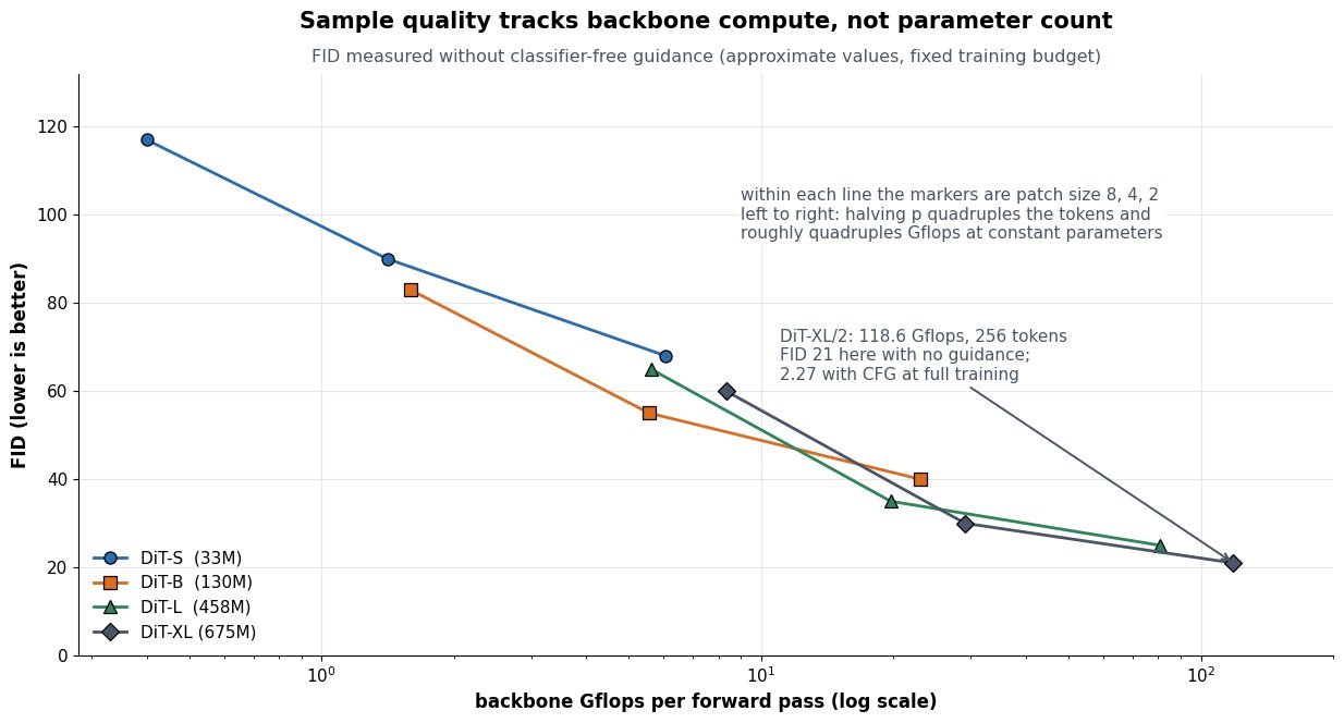
Log-x line chart of FID against backbone Gflops for DiT-S, DiT-B, DiT-L and DiT-XL, each line connecting patch sizes 8, 4 and 2, showing FID falling monotonically as Gflops rise

Figure 2: Approximate FID against backbone Gflops at a fixed 400K-step training budget and without classifier-free guidance, which is why the absolute values sit far above the guided FID 2.27 quoted for the fully trained DiT-XL/2. What matters here is the trend: quality tracks compute rather than parameter count, so DiT-B with $p = 2$ can outrun DiT-L with $p = 8$ despite having far fewer parameters.

Property	DiT	U-Net (ADM, LDM, SDXL)
Spatial handling	One fixed-length token sequence, no resampling and no skips	Resolution pyramid 32 → 16 → 8 → 4 → 8 → 16 → 32 with skip connections
Conditioning path	adaLN-Zero: per-block scale, shift, and zero-initialized residual gate from $c$	Timestep embedding added inside ResBlocks, text or class via cross-attention
Compute knobs	Depth, width, and patch size; patch size changes Gflops at constant parameters	Channel multipliers, blocks per level, and which levels get attention
Inductive bias	Minimal beyond positional embeddings, so it needs more data and compute to pay off	Strong locality and multi-scale bias, sample-efficient at small budgets
Cost as resolution grows	$O(T^2 d)$ attention, so latent compression and patch size are load-bearing	Convolutions grow linearly in pixels; attention only at low-resolution levels
Scaling behavior	FID a smooth decreasing function of Gflops, easy to extrapolate	Gains depend on hand-designed schedules and saturate less predictably

One caveat when quoting numbers in an interview: FID is only comparable within a fixed evaluation protocol. The headline 2.27 comes from the fully trained DiT-XL/2 sampled with classifier-free guidance at scale 1.5; the same checkpoint sampled without guidance lands near 9.6, and the scaling sweep above uses a much shorter 400K-step budget with no guidance at all. Guidance, training steps, sampler, and step count all move the number by more than the architectural gap being discussed, so state the protocol alongside the score.

August 16, 2026

DL0104 Score-Based Diffusion

What is the score-based / score-matching interpretation of diffusion models, as used in systems like Stable Diffusion?

Answer

The score-based view says a diffusion model never learns a density; it learns the score, the gradient of the log density $s(x) = \nabla_x \log p(x)$ . This is attractive because the gradient annihilates the intractable normalizing constant: if $p(x) = e^{-E(x)}/Z$ then $\nabla_x \log p(x) = -\nabla_x E(x)$ with no $Z$ anywhere, so an unnormalized energy model becomes trainable. Direct score matching still needs the intractable $\nabla_x \log p_{\text{data}}(x)$ , and the fix is denoising score matching: perturb the data with a known Gaussian kernel, and the score of the perturbed conditional is available in closed form, which reduces the loss to predicting the noise that was added. Because a single small noise level leaves the score undefined off the data manifold and unreliable in low-density regions, the model is trained over a continuum of noise levels, which turns into the forward SDE of Song et al. and makes sampling the simulation of a reverse-time SDE or its deterministic probability-flow ODE. The punchline is that DDPM’s noise-prediction network is the same object in different clothing: $s_\theta(x_t,t) = -\epsilon_\theta(x_t,t)/\sigma_t$ , so the discrete-time denoising story and the continuous-time score story are two parameterizations of one model.

(1) Model The Gradient, Not The Density: learning $\nabla_x \log p(x)$ removes the partition function, so the network output is an unconstrained vector field of the same shape as the data.
(2) Denoising Score Matching Makes It Tractable: Vincent’s identity shows that regressing onto $\nabla_{x_t}\log p(x_t \mid x_0)$ has the same minimizer as matching the true marginal score, and that target is just the scaled added noise.
(3) Multiple Noise Scales Are Essential: real data lies near a low-dimensional manifold where the score is ill-defined, and large noise levels smooth the density so the vector field is informative everywhere and connects separated modes.
(4) Sampling Is Numerical Integration: annealed Langevin dynamics, the reverse SDE, and the probability-flow ODE all consume only the learned score; the ODE additionally gives exact likelihoods and deterministic, invertible latents.
(5) Unifies VE And VP Diffusions: NCSN’s variance-exploding noise ladder and DDPM’s variance-preserving chain are two discretizations of the same SDE family, differing in $f$ , $g$ , and the loss weighting $\lambda_t$ .

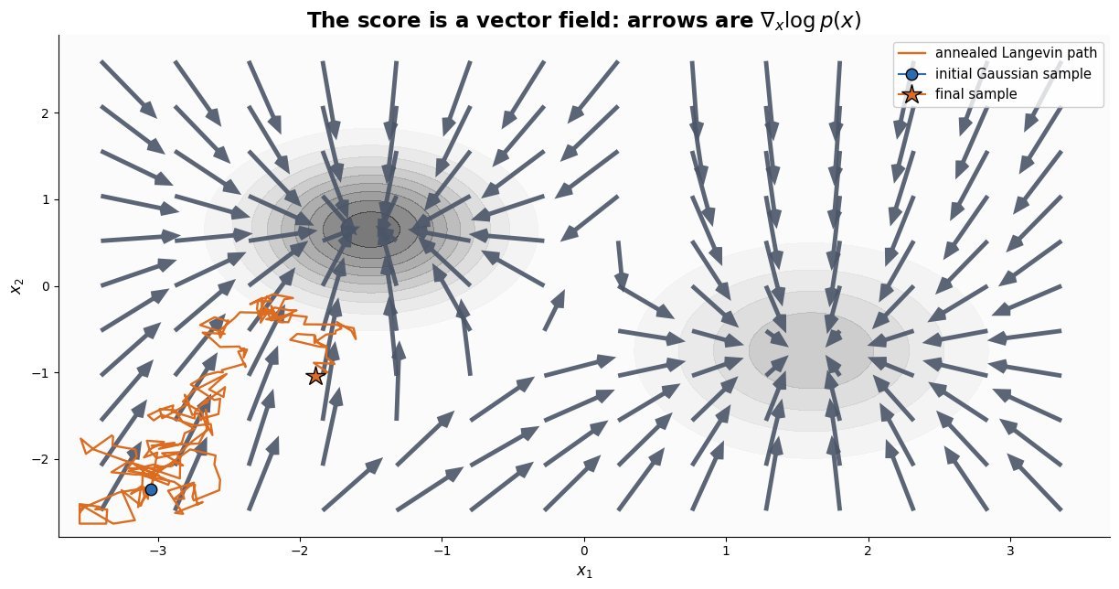
The geometric picture is worth holding onto. The score at a point is the direction of steepest increase in log density, so the learned field points from wherever you are toward nearby high-probability regions, and its magnitude grows as you move into the tails. Sampling then means dropping a Gaussian sample somewhere in space and following that field while injecting just enough noise to keep the chain from collapsing onto a single mode. The reason this needs annealing is that a score trained only at tiny noise is accurate on the data manifold and near-arbitrary far from it, where every initial sample actually starts.

Contour plot of a two-mode density with an overlaid arrow field pointing toward the modes, and a jagged Langevin sampling path starting in the empty lower-left corner and ending inside the left mode

Figure 1: The learned score is a vector field pointing toward high-density regions; a Langevin chain follows it from a random start and ends up distributed according to $p(x)$ , never evaluating the density itself.

Mathematical Formulation:
$s_\theta(x,t) \approx \nabla_x \log p_t(x)$
$x_t = \alpha_t x_0 + \sigma_t \epsilon$
$\nabla_{x_t} \log p(x_t \mid x_0) = -\frac{\epsilon}{\sigma_t}$
$\mathcal{L}(\theta) = \mathbb{E}\left[ \lambda_t \left\| s_\theta(x_t,t) + \frac{\epsilon}{\sigma_t} \right\|^2 \right]$
$dx = f(x,t)\,dt + g(t)\,dw$
$dx = \left[ f - g^2 s_\theta \right] dt + g\,d\bar{w}$
$dx = \left[ f - \tfrac{1}{2} g^2 s_\theta \right] dt$
$s_\theta(x_t,t) = -\frac{\epsilon_\theta(x_t,t)}{\sigma_t}$

Where:

$s_\theta(x,t)$ is the network output, a vector with the same shape as $x$ , approximating the score of the perturbed marginal $p_t$ .
$x_0$ is a clean data point, $x_t$ its noisy version, and $\epsilon \sim \mathcal{N}(0,I)$ the Gaussian draw.
$\alpha_t$ and $\sigma_t$ define the noise schedule; variance-preserving keeps $\alpha_t^2 + \sigma_t^2 = 1$ , variance-exploding fixes $\alpha_t = 1$ and grows $\sigma_t$ .
$t \in [0,T]$ indexes the noise level, with $p_T$ essentially pure Gaussian noise; $\lambda_t$ is the loss weighting, and the choice $\lambda_t = \sigma_t^2$ turns the objective into the plain noise-prediction MSE.
$f(x,t)$ is the drift and $g(t)$ the diffusion coefficient of the forward SDE; $w$ is a Wiener process and $\bar{w}$ its reverse-time counterpart, so the second SDE is integrated from $t = T$ down to $t = 0$ .
The final line is the reparameterization identity linking the score view to DDPM’s $\epsilon_\theta$ ; required initial condition for sampling: $x_T \sim \mathcal{N}(0, \sigma_T^2 I)$ for the VE case.

Three panels showing the same two-mode density smoothed by increasing Gaussian noise, with score arrows that are confined near the modes at small noise and fill the whole plane at large noise

Figure 2: Why a ladder of noise levels is required: at $\sigma = 0.05$ the score carries no usable signal away from the data, while at $\sigma = 1.5$ the smoothed field points inward from everywhere and bridges the two modes.

Property	Score SDE (VE, NCSN)	DDPM (VP, noise-pred)	Flow matching
Network output	Score, magnitude scales like 1/sigma_t	Unit-variance noise estimate	Velocity field of a probability path
Corruption	Add noise, variance grows to data scale	Shrink signal, keep total variance at 1	Straight interpolation between data and noise
Loss	Weighted denoising score matching	Same loss with weighting sigma_t squared	Regression onto the conditional velocity
Sampler	Annealed Langevin or predictor-corrector	Ancestral chain, or DDIM as an ODE	ODE solver on a near-straight path
Exact likelihood	Yes, via the probability-flow ODE	Only an ELBO in discrete time	Yes, continuous normalizing flow change of variables

August 16, 2026

DL0103 Stable Diffusion Latent Space

What is latent diffusion, and why does Stable Diffusion run diffusion in a VAE latent space?

Answer

Latent diffusion splits image generation into two stages that are trained separately: a convolutional autoencoder first compresses pixels into a small spatial latent, and the diffusion model then learns the noise process entirely inside that latent grid. Stable Diffusion uses a KL-regularized VAE with downsampling factor $f = 8$ , so a $512 \times 512 \times 3$ image becomes a $64 \times 64 \times 4$ latent: 786,432 values collapse to 16,384, a 48x reduction in the tensor the U-Net has to denoise. The motivation is that the two stages solve different problems. Pixel-space diffusion wastes most of its capacity and most of its training steps modeling imperceptible high-frequency detail, exactly the information a perceptual codec throws away for free; the autoencoder handles that perceptual compression once, and the diffusion model is left with the semantic compression problem of arranging layout, objects, and style. The compute argument is even stronger than the 48x suggests, because the U-Net contains self-attention: token count drops from 262,144 to 4,096, so any $O(N^2)$ attention block gets $f^4 = 4096$ times cheaper. That is what turned high-resolution text-to-image training from a large-cluster project into something reproducible on modest hardware, and what makes 50-step sampling on a consumer GPU feasible at all.

(1) Two-Stage Factorization: the autoencoder is trained first and then frozen; the diffusion model never sees a pixel, and the decoder is invoked exactly once at the end of sampling.
(2) Quadratic Savings On Attention: the latent grid has $f^2$ fewer positions, so convolutions get $f^2$ cheaper and self-attention gets roughly $f^4$ cheaper.
(3) It Is Not A Generative VAE: the KL weight is tiny (on the order of $10^{-6}$ ) and the reconstruction loss adds LPIPS plus a patch discriminator, so the encoder behaves as a sharp lossy codec rather than a prior you would ever sample from.
(4) Latent Scaling Matters: encoder outputs are multiplied by a constant (0.18215 for SD 1.x, 0.13025 for SDXL) so the latent has roughly unit variance and the standard noise schedule reaches a true $\mathcal{N}(0, I)$ terminal state.
(5) Cheap Conditioning And Editing: CLIP text embeddings enter through cross-attention at every latent resolution, and img2img, inpainting, and ControlNet all operate on the same small latent grid.
(6) The Decoder Is The Fidelity Ceiling: nothing the diffusion model does can recover detail the 4-channel latent discarded, which is why small text, fine textures, and tiny faces degrade first.

Pipeline diagram: a 512 by 512 by 3 image enters a VAE encoder producing a 64 by 64 by 4 latent, an iterative denoising U-Net conditioned by CLIP text cross-attention operates on the latent for T steps, and a VAE decoder maps the result back to pixels

Figure 1: Training and sampling both live in the 4,096-token latent grid; the frozen encoder and decoder are the only components that ever touch the 262,144-pixel image, and text conditioning enters the denoiser through cross-attention.

The choice of $f$ is a genuine trade-off rather than a free win. The original LDM ablations show that $f \in \{4, 8\}$ is the sweet spot: at $f = 1$ or $2$ training is slow because the model is still doing perceptual compression itself, while at $f = 32$ with only 4 channels the autoencoder becomes the bottleneck and sample quality saturates no matter how long the diffusion model trains. Channel count $c$ is the other lever, and it is the one that later models moved: SD3 and Flux keep $f = 8$ but raise the latent to 16 channels, quartering the compression ratio from 48 to 12 to trade a little step cost for a much better reconstruction ceiling on text and fine structure. A practical consequence of the frozen-codec design is that latents are model-specific: an SDXL latent decoded by an SD 1.5 decoder produces color-shifted garbage, because the two autoencoders were trained with different scaling and channel statistics.

Mathematical Formulation:
$z_0 = s \cdot \mathcal{E}(x)$
$\hat{x} = \mathcal{D}(z_0 / s)$
$z_t = \sqrt{\bar\alpha_t}\, z_0 + \sqrt{1 - \bar\alpha_t}\, \epsilon$
$\mathcal{L} = \mathbb{E}\left[\lVert \epsilon - \epsilon_\theta(z_t, t, \tau(y)) \rVert_2^2\right]$
$\rho = \frac{3 f^2}{c}$
$\rho = \frac{3 \cdot 64}{4} = 48$

Where:

$x \in \mathbb{R}^{H \times W \times 3}$ is the image and $\hat{x}$ its reconstruction; $z_0 \in \mathbb{R}^{h \times w \times c}$ is the clean latent with $h = H/f$ and $w = W/f$ .
$\mathcal{E}$ and $\mathcal{D}$ are the frozen VAE encoder and decoder, and $s$ is the latent scaling constant that normalizes the variance.
$t \in \{1, \ldots, T\}$ is the timestep, $\bar\alpha_t$ the cumulative noise schedule, and $\epsilon \sim \mathcal{N}(0, I)$ the sampled Gaussian noise.
$\epsilon_\theta$ is the latent denoiser (U-Net in SD 1.x and SDXL, a transformer in DiT-style successors), and $\tau(y)$ is the text-encoder output injected by cross-attention.
$f$ is the spatial downsampling factor and $c$ the latent channel count; $\rho$ is the element compression ratio, which is 48 for $f = 8, c = 4$ and 12 for $c = 16$ .
Required initial condition at sampling: $z_T \sim \mathcal{N}(0, I)$ on the latent grid, which only holds if $s$ was applied and $\bar\alpha_T \approx 0$ .

Log-scale bar chart of self-attention cost reduction relative to pixel space at 512 by 512 resolution: factor 1 for pixel space with 262144 tokens, 256 for f equals 4, 4096 for f equals 8, and 65536 for f equals 16

Figure 2: Because self-attention scales as $O(N^2)$ in the token count, compressing by $f$ cuts attention cost by $f^4$ ; the $f = 8$ setting used by Stable Diffusion buys a 4096x reduction while keeping the decoder’s reconstruction error acceptable.

Property	Latent diffusion (Stable Diffusion)	Single-stage pixel diffusion	Cascaded pixel diffusion
Where noise is added	A 64x64x4 VAE latent	Directly on RGB pixels at full resolution	Pixels at 64×64, then two super-resolution diffusion stages
Denoiser input size at 512×512	4,096 tokens, 16,384 values	262,144 tokens, 786,432 values	4,096 tokens in the base model, full resolution in the last upsampler
Training and sampling cost	Lowest; one model, attention roughly 4096x cheaper per block	Highest; attention is usually dropped or windowed to stay tractable	Moderate but multiplied by the number of stages
Fidelity ceiling	Bounded by decoder reconstruction error, independent of training length	No codec bottleneck; exact pixel modeling is possible	No codec bottleneck, but upsamplers can hallucinate detail
Typical failure mode	Mangled small text, smeared fine texture, artifacts on tiny faces	Under-trained global structure for a fixed compute budget	Error accumulation and train/test mismatch between stages

August 16, 2026

DL0102 Diffusion vs GAN vs VAE

Explain the fundamental principles of Diffusion Models, and compare their pros and cons with GANs, VAEs, and Flow-based models.

Answer

A diffusion model defines a fixed forward process that gradually corrupts data into Gaussian noise over $T$ steps, then learns the reverse process that removes a little noise at a time. The forward chain has no parameters and admits a closed form, so training reduces to a plain regression: sample a clean image $x_0$ , sample a timestep $t$ and noise $\epsilon$ , build the noisy state $x_t$ , and ask the network to predict $\epsilon$ . This denoising objective is a weighted variational bound on the log-likelihood and is also equivalent to score matching, which is why the same network can be plugged into an SDE or ODE sampler. The practical consequence is that diffusion buys stable training and excellent mode coverage at the price of many network evaluations per sample, whereas a GAN generates in one forward pass but fights an unstable min-max game, a VAE trains stably but produces blurry samples under a Gaussian decoder, and a normalizing flow gives exact likelihoods but pays for invertibility with architectural constraints and parameter count.

(1) Fixed Corruption, Learned Reversal: only the reverse direction has parameters, so there is no adversary and no discriminator to balance, which removes the main source of GAN training instability.
(2) Closed-Form Training Target: because $q(x_t \mid x_0)$ is Gaussian, any timestep can be sampled directly without simulating the chain, making each training step $O(1)$ in $T$ .
(3) Score Interpretation: the noise predictor is a rescaled estimate of $\nabla_{x_t}\log q(x_t)$ , which links diffusion to Langevin dynamics and to probability-flow ODE samplers such as DDIM.
(4) Sampling Is The Bottleneck: quality scales with the number of function evaluations, so a 1000-step DDPM sampler costs three orders of magnitude more compute per image than a GAN generator.
(5) Coverage Versus Speed: the likelihood-flavored objective penalizes dropped modes, which is exactly the failure GANs are known for, so the two families sit on opposite corners of the quality/diversity/speed trade-off.

Diagram of a diffusion chain: five states from a clean image to pure noise, with upper arrows showing the fixed forward noising process q and lower arrows showing the learned reverse denoiser p theta, plus a dashed arc marking the closed-form jump from x0 to any xt

Figure 1: The forward process is fixed and parameter-free, and the dashed arc is the closed form that lets training jump straight to any $x_t$ ; every arrow in the lower reverse path costs one network evaluation at sampling time.

The four families differ mostly in how they pay for tractability. A VAE keeps an explicit encoder and decoder and optimizes a lower bound, so the mismatch between the true posterior and the Gaussian approximation shows up as blur and posterior collapse. A normalizing flow refuses any approximation and computes exact likelihoods, but every layer must be invertible with a cheap Jacobian determinant, which caps expressiveness per parameter. A GAN drops likelihood entirely and optimizes a discriminator-defined divergence, which produces sharp samples in one step but offers no signal that the whole data distribution is covered. Diffusion sidesteps all three constraints by turning generation into a long sequence of easy denoising problems, and then spends compute at inference to pay for it.

Mathematical Formulation:
$q(x_t \mid x_{t-1}) = \mathcal{N}(x_t; \sqrt{1-\beta_t}\, x_{t-1}, \beta_t I)$
$\bar{\alpha}_t = \prod_{s=1}^{t} (1 - \beta_s)$
$x_t = \sqrt{\bar{\alpha}_t}\, x_0 + \sqrt{1 - \bar{\alpha}_t}\, \epsilon$
$\mathcal{L}_{\text{simple}} = \mathbb{E}_{t, x_0, \epsilon} [ \| \epsilon - \epsilon_\theta(x_t, t) \|^2 ]$
$s_\theta(x_t, t) = -\frac{\epsilon_\theta(x_t, t)}{\sqrt{1 - \bar{\alpha}_t}}$

Where:

$x_0$ is a clean data sample and $x_t$ the noised state at step $t$ , with $x_T$ approximately standard Gaussian.
$\epsilon \sim \mathcal{N}(0, I)$ is the injected noise and $\epsilon_\theta$ the learned noise predictor with parameters $\theta$ .
$t \in \{1, \ldots, T\}$ is sampled uniformly during training, and $s$ indexes the product defining the cumulative signal retention.
$\beta_t$ is the noise schedule, typically small and increasing, and $\bar{\alpha}_t$ is the cumulative signal factor giving signal-to-noise ratio $\bar{\alpha}_t / (1 - \bar{\alpha}_t)$ .
$s_\theta$ is the implied score function, the quantity an SDE or probability-flow ODE sampler integrates.
Required initial condition: sampling starts from $x_T \sim \mathcal{N}(0, I)$ , which is only valid if the schedule drives $\bar{\alpha}_T$ to (near) zero.

Property	Diffusion	GAN	VAE	Normalizing Flow
Training objective	Denoising regression on a fixed forward process, no adversary	Min-max game against a discriminator	ELBO: reconstruction plus KL to the prior	Exact log-likelihood via change of variables
Network calls per sample	10 to 1000, or 1 to 4 after distillation	1	1	1
Sample fidelity	State of the art for images, video, and audio	Very sharp, still strong under a one-step budget	Blurry with a Gaussian decoder	Below GAN and diffusion at equal compute
Mode coverage	Broad, the objective penalizes missing mass	Mode collapse is the classic failure	Broad but over-smoothed	Broad, likelihood forbids ignoring regions
Density estimate	Bound or ODE-based estimate, not exact in closed form	None	Lower bound only	Exact and tractable
Architecture constraint	Free, any denoiser such as a U-Net or a DiT	Free	Free	Invertible layers with cheap Jacobian determinant
Typical failure	Slow sampling, schedule and guidance artifacts	Unstable training, collapsed diversity	Blur and posterior collapse	Very large models for modest sample quality

Triangle diagram of the generative learning trilemma with vertices high sample quality, fast sampling, and mode coverage; GAN sits on the quality-speed edge, VAE and normalizing flow on the speed-coverage edge, and diffusion on the quality-coverage edge

Figure 2: The generative learning trilemma: each family wins two corners and pays on the third, and most modern work on diffusion (distillation, consistency training, rectified flow) is an attempt to drag it toward the fast-sampling corner without losing coverage.

August 16, 2026

DL0101 GAN Loss Functions

What loss functions do the GAN generator and discriminator optimize?

Answer

The discriminator optimizes an ordinary binary cross-entropy objective: label real samples 1, generated samples 0, and minimize the negative log-likelihood of that two-class problem. The generator is defined by the same value function played in the opposite direction, so the textbook formulation is the minimax game $\min_{G} \max_{D} V(D,G)$ , but almost nobody implements the generator that way. Minimizing $\log(1 - D(G(z)))$ saturates exactly when the generator is bad, which is precisely when it needs signal, so Goodfellow’s original paper already proposed the non-saturating form: maximize $\log D(G(z))$ , or equivalently minimize $-\log D(G(z))$ . Both variants share the same fixed point, where the optimal discriminator is $D^{*}(x) = p_{r}(x)/(p_{r}(x)+p_{g}(x))$ and the outer objective reduces to the Jensen-Shannon divergence between data and model. In current practice the exact loss shape matters less than the regularizer attached to it, and the common defaults are the non-saturating logistic loss or the hinge loss combined with an R1 gradient penalty on real data.

(1) Discriminator Is Just A Classifier: its loss is standard BCE over a batch of half real and half fake samples, so any logit-based classification loss can be dropped in without changing the game structure.
(2) Saturating Vs Non-Saturating Generator: the two forms have identical optima but very different gradient magnitudes; the non-saturating loss keeps a large gradient when $D(G(z))$ is near 0.
(3) Optimal Discriminator Reveals A Divergence: substituting $D^{*}$ turns the value function into $2\,\mathrm{JSD}(p_{r} \,\|\, p_{g}) - \log 4$ , which is why a perfect discriminator gives no useful gradient on disjoint supports.
(4) Alternatives Change The Metric: LSGAN uses a squared error, WGAN replaces the classifier with a 1-Lipschitz critic estimating the Earth-Mover distance, and hinge loss caps the penalty once a margin is met.
(5) Regularization Dominates Stability: zero-centered gradient penalties such as R1 are what make training converge locally, and swapping loss families with the same regularizer usually moves FID far less than practitioners expect.

Two panel chart: left panel plots the saturating generator loss log of one minus D and the non-saturating loss minus log D against the discriminator score on a fake sample, right panel plots the magnitude of their gradients on a logarithmic axis showing the non-saturating gradient is far larger when the score is near zero

Figure 1: Early in training the discriminator confidently rejects fakes, so $D(G(z))$ sits near 0. At $D(G(z)) = 0.05$ the saturating loss supplies a gradient magnitude of 1.05 while the non-saturating loss supplies 20, about 19x more signal in exactly the regime where the generator is weakest.

Mathematical Formulation:
$\min_{G} \max_{D} V(D, G)$
$V(D,G) = \mathbb{E}_{x \sim p_{r}}[\log D(x)]$
$+ \mathbb{E}_{z \sim p_{z}}[\log (1 - D(G(z)))]$
$\mathcal{L}_{G}^{\mathrm{sat}} = \mathbb{E}_{z}[\log (1 - D(G(z)))]$
$\mathcal{L}_{G}^{\mathrm{ns}} = -\mathbb{E}_{z}[\log D(G(z))]$
$D^{*}(x) = \frac{p_{r}(x)}{p_{r}(x) + p_{g}(x)}$
$V(D^{*}, G) = 2\,\mathrm{JSD}(p_{r} \,\|\, p_{g}) - \log 4$

Where:

$V(D,G)$ is the value function; the discriminator maximizes it and the generator minimizes it, so $\mathcal{L}_{D} = -V$ is the batch-level binary cross-entropy actually coded up.
$x \sim p_{r}$ is a real sample and $D(x) \in [0,1]$ is the estimated probability that its input is real.
$z \sim p_{z}$ is a latent drawn from a fixed prior, usually $\mathcal{N}(0, I)$ ; $G(z)$ is the generated sample and $p_{g}$ the distribution it induces.
$\mathcal{L}_{G}^{\mathrm{sat}}$ is the literal minimax generator loss and $\mathcal{L}_{G}^{\mathrm{ns}}$ the non-saturating heuristic; they share the same optimum but differ in gradient scale by a factor of $(1 - D)/D$ .
$D^{*}$ is the optimal discriminator for a fixed $G$ , obtained by maximizing the integrand pointwise; it equals $1/2$ everywhere when $p_{g} = p_{r}$ .
$\mathrm{JSD}$ is bounded in $[0, \log 2]$ , so $V(D^{*},G)$ ranges over $[-\log 4, 0]$ and hits its global minimum $-\log 4 \approx -1.386$ only at $p_{g} = p_{r}$ .
Practical condition: $D^{*}$ is never reached, since the discriminator takes $k$ steps (typically $k = 1$ ) per generator step, and the whole derivation assumes optimization in function space rather than over network parameters.

The main alternatives keep the same alternating structure and change only the per-sample penalty. LSGAN replaces the log with a squared error, which pushes fake samples toward the decision boundary and stops the loss from flattening, at the cost of also penalizing samples that are already comfortably on the correct side. WGAN drops the sigmoid entirely: the critic maximizes $\mathbb{E}[D(x)] - \mathbb{E}[D(G(z))]$ under a 1-Lipschitz constraint, enforced in WGAN-GP by a two-sided penalty on the gradient norm at interpolated points, and the generator simply maximizes $\mathbb{E}[D(G(z))]$ . Hinge loss, the default in BigGAN and many diffusion-era discriminators, uses $\max(0, 1 - D(x))$ on reals and $\max(0, 1 + D(G(z)))$ on fakes, so a correctly classified sample beyond the margin contributes exactly zero gradient and the discriminator stops overfitting easy examples. Independently of the family chosen, the R1 penalty $\frac{\gamma}{2}\mathbb{E}_{x \sim p_{r}}[\|\nabla_{x} D(x)\|^{2}]$ is what turns the local dynamics from oscillatory into convergent.

Line chart of the discriminator loss contributed by a single fake sample as a function of its logit, comparing the smooth softplus curve of binary cross-entropy, the piecewise linear hinge loss that becomes exactly zero below minus one, and the unbounded linear Wasserstein critic loss

Figure 2: Loss contributed by one fake sample as a function of its logit $t$ . BCE uses $\log(1 + e^{t})$ and decays smoothly but never quite to zero, hinge is exactly flat once the sample clears the $-1$ margin, and the Wasserstein critic stays linear so it never saturates and must be constrained by a Lipschitz penalty.

Property	Non-saturating BCE	Hinge	WGAN-GP
Discriminator term on a fake	softplus of the logit, smooth and always positive	max(0, 1 + logit), exactly zero past the margin	the raw critic score, unbounded and linear
Generator term	minus log of the fake probability	minus the critic score, no hinge applied	minus the critic score
Behavior when D wins	gradient shrinks but stays usable via the non-saturating form	D stops learning from easy samples, which limits overfitting	score gap keeps growing, so the generator still gets signal
Extra cost per step	none beyond an optional R1 penalty, often lazily applied every 16 steps	same as BCE	a double backward pass for the penalty plus roughly 5 critic steps per generator step
Typical use	StyleGAN family with R1, and most adversarial auxiliary losses	BigGAN, SAGAN, and many feature-space discriminators	settings where a meaningful loss-versus-quality correlation is wanted

August 16, 2026