Author: admin

ML0083 Weight Decay

What is weight decay in neural network training, and how does it affect model parameters?

Answer

Weight decay multiplies every weight by a factor slightly below one at each step, so parameters continuously shrink toward zero unless the data gradient pushes them back up. The equilibrium effect: only directions where the loss gradient persistently outweighs the decay survive with large magnitude, while noise-fitting directions get eroded, which is exactly the capacity control we want. For plain SGD, weight decay is mathematically identical to adding an L2 penalty to the loss. For adaptive optimizers like Adam it is not, because the L2 gradient gets rescaled per-parameter along with everything else; AdamW fixes this by decoupling the decay from the adaptive update, and is now the default recipe for training transformers.

(1) Mechanics: each step shrinks weights multiplicatively before (or alongside) the gradient step, so unneeded complexity decays exponentially while useful weights are constantly re-earned from the data gradient.
(2) SGD Equivalence and Its Caveat: for SGD, weight decay with rate lambda equals L2 regularization with coefficient lambda/alpha, so the two are coupled through the learning rate; retuning alpha silently retunes your regularization.
(3) AdamW Fix: Loshchilov and Hutter showed Adam’s adaptive scaling under-regularizes high-gradient weights when L2 is folded into the loss; AdamW applies decay outside the adaptive step, and PyTorch’s AdamW defaults to a weight decay of 0.01.

Elliptical loss contours centered away from the origin, a dashed L2 constraint circle around the origin, and the regularized optimum where the circle touches a contour

Figure 1: The geometric view: the unregularized optimum sits far from the origin; weight decay pulls the solution to where the smallest L2 ball first touches the loss contours, trading a little fit for a lot of magnitude.

The Adam subtlety is worth understanding precisely, because it is a favorite interview trap. In Adam, every component of the gradient, including the penalty’s contribution, is divided by the square root of its running second moment. Parameters with historically large data gradients therefore experience a heavily damped regularization force, which is backwards: the parameters the optimizer is already moving hardest are the ones the penalty reaches least. Note the denominator tracks the second moment of the gradient, not the weight’s own magnitude, so the effect is uneven regularization across parameters rather than a simple “big weights decay less” rule. AdamW removes the penalty from the adaptive gradient entirely and applies it as a direct multiplicative shrink, restoring uniform, controllable decay, which is why nearly every modern pretraining run (GPT-style models included) specifies AdamW.

Weight norm over training steps: no decay grows steadily, Adam plus L2 barely shrinks it, AdamW settles at a lower plateau

Figure 2: The decoupling effect: with no decay the weight norm grows unchecked; Adam with L2 in the loss barely contains it because the penalty is adaptively rescaled; AdamW’s decoupled decay settles at a controlled plateau.

Mathematical Formulation:
$\theta_{t+1} = (1 - \lambda)\,\theta_t - \alpha\, \nabla f_t(\theta_t)$
$f^{reg}_t(\theta) = f_t(\theta) + \frac{\lambda'}{2}\,\|\theta\|^2, \qquad \lambda' = \lambda / \alpha$

Where:

$\theta_t$ collects all parameters at step $t$ , $\alpha$ is the learning rate, and $\lambda$ is the per-step decay rate.
$f_t$ is the minibatch loss; the $(1 - \lambda)$ factor is the multiplicative shrink applied every step.
$\lambda' = \lambda/\alpha$ is the L2 coefficient that makes the two formulations equivalent for SGD, exposing the coupling: change the learning rate and the effective regularization changes too (this equivalence fails for adaptive optimizers, hence AdamW).

Aspect	L2 in the Loss (Adam)	Decoupled Decay (AdamW)
Where Applied	Penalty gradient added to the loss gradient	Direct multiplicative shrink, outside the adaptive step
Adaptive Scaling	Penalty is divided by sqrt(v), so large-gradient weights decay least	Decay is uniform across parameters
Hyperparameter Coupling	Effective regularization entangled with learning rate and gradient scale	Decay rate tuned independently of learning rate
Default Use	Legacy; PyTorch Adam weight_decay argument is actually L2	Standard for transformer pretraining; PyTorch default 0.01

August 11, 2026

ML0082 XGBoost Improves Gradient Boosting

How does XGBoost improve upon the classical gradient-boosted decision tree algorithm?

Answer

XGBoost keeps the sequential additive recipe of classical gradient boosting but upgrades it on three axes. First, optimization: it fits each tree with a second-order Taylor approximation of the loss, using both gradients and Hessians, so leaf weights and split gains are Newton-style steps instead of plain gradient steps. Second, regularization: the objective explicitly penalizes the number of leaves and the squared leaf weights, which prunes weak splits analytically. Third, systems: sparsity-aware split finding, a weighted quantile sketch for approximate splits, and cache-aware block layouts let it scale to billions of examples. The result dominated competitions: 17 of the 29 winning solutions published on Kaggle’s blog in 2015 used XGBoost.

(1) Second-Order Optimization: gradients alone say which way is downhill; Hessians say how curved the surface is, so XGBoost computes closed-form optimal leaf weights and exact split gains per candidate split.
(2) Regularized Objective: the penalty on leaf count and weight magnitude means a split must beat an explicit complexity cost to survive, a built-in analogue of pruning that classical GBDT lacks.
(3) Systems Engineering: default directions for missing values, approximate split proposals from weighted quantiles, and out-of-core cache-aware blocks deliver the reported 10x-plus speedups that made it the industry default.

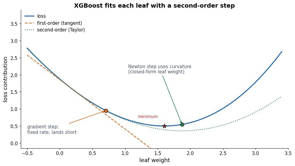
One-dimensional loss curve with a gradient-only step undershooting the minimum while a second-order Newton step, using curvature, lands near it

Figure 1: Why the Hessian helps: a first-order step moves along the tangent and misses the valley; a second-order step accounts for curvature (dashed parabola) and lands near the minimizer, which is what closed-form leaf weights do for every leaf.

The second-order view also explains where the regularization bites. Once you collect all examples routed to a leaf, the objective contribution of that leaf is a one-dimensional quadratic in its weight, whose closed-form minimizer shrinks toward zero as the penalty grows. Splits are scored by how much they reduce the total objective including the per-leaf cost, so a split that adds two leaves must overcome an explicit gamma toll twice. Classical GBDT instead fits trees to raw gradients and controls complexity only indirectly through depth caps and shrinkage.

Mathematical Formulation:
$\mathcal{L}^{(t)} \simeq \sum_{i=1}^{N} \left[ g_i f_t(x_i) + \frac{1}{2} h_i f_t^2(x_i) \right] + \Omega(f_t)$
$\Omega(f) = \gamma T + \frac{1}{2}\lambda \sum_{j=1}^{T} w_j^2$
$w_j^* = -\frac{G_j}{H_j + \lambda}$

Where:

$g_i$ and $h_i$ are the first and second derivatives of the per-example loss at the current prediction; $f_t$ is the new tree.
$\Omega(f)$ is the regularizer: $\gamma$ charges per leaf ( $T$ leaves) and $\lambda$ penalizes squared leaf weights $w_j$ .
$G_j, H_j$ are the sums of $g_i, h_i$ over the examples routed to leaf $j$ , and $w_j^*$ is the closed-form optimal leaf weight; larger $\lambda$ shrinks every leaf toward zero.

Aspect	Classical GBDT	XGBoost
Loss Information	First-order gradients (residuals)	Gradients + Hessians (second-order Taylor)
Regularization	Indirect: depth caps, shrinkage, subsampling	Explicit: gamma on leaf count, lambda on leaf weights
Split Finding	Exact scan or basic histograms	Weighted quantile sketch + sparsity-aware defaults
Scale	In-memory, single machine	Cache-aware blocks, out-of-core, distributed
Track Record	Strong but slow at scale	17 of 29 Kaggle 2015 winning solutions; every KDDCup 2015 top-10 team

August 11, 2026

ML0081 Gradient Boosting vs Random Forest

How do gradient-boosted decision trees work, and how do they differ from random forests?

Answer

Gradient boosting builds an additive ensemble sequentially: each new tree is fit to the negative gradient of the loss with respect to the current ensemble’s predictions (for squared error, the residuals), then added in with a small learning rate. The ensemble is a directed attack on bias; every stage shrinks whatever error remains. A random forest does the opposite: it grows many deep trees independently on bootstrap samples with random feature subsets and averages their votes, which attacks variance. So boosting uses shallow trees, a learning rate, and sequence, while bagging uses deep trees, randomness, and parallel averaging.

(1) Sequential Residual Fitting: tree m targets the current gradient (pseudo-residuals); with squared loss this is literally y minus the running prediction, and shrinkage keeps any single tree from dominating.
(2) Bias vs Variance: boosting reduces bias stage by stage but can chase noise if run long or deep; random forests reduce variance by decorrelating many overfit trees, but their bias is roughly that of one tree.
(3) Modern Refinement: Yandex showed classic gradient boosting leaks target information into its own gradients (prediction shift), and CatBoost’s ordered boosting fixes it by computing each example’s gradient from a model trained only on earlier examples in a random permutation.

Three panels: initial prediction is flat with large residuals; after adding tree one the curve follows the data and residuals shrink; after tree two the fit is close and residuals are small

Figure 1: Stage-wise fitting: each new tree targets the residuals (orange stems) left by the current ensemble, so the prediction curve (blue) bends toward the data a little at every stage.

Structurally, the two ensembles could not be more different. A random forest is embarrassingly parallel: tree one and tree one hundred do not know each other, so you can train them on separate machines and the average cancels their individual overfitting. Gradient boosting is an inherently sequential chain: tree one hundred is defined by the mistakes of the previous ninety-nine, which buys accuracy on structured tabular data but makes training serial and makes the model sensitive to label noise, because late-stage trees are explicitly trained to fit whatever is left, including the noise.

Side-by-side schematics: random forest trains deep trees in parallel on bootstrap samples and averages votes; gradient boosting trains shallow trees in a chain where each consumes the previous ensemble's residuals

Figure 2: Parallel averaging vs sequential correction: the forest’s trees are independent and deep, the boosted trees are shallow and chained through residuals, with a learning rate throttling each contribution.

Mathematical Formulation:
$F_m(x) = F_{m-1}(x) + \nu\, h_m(x)$
$r_{i,m} = -\left[\frac{\partial\, \ell(y_i, F(x_i))}{\partial\, F(x_i)}\right]_{F = F_{m-1}}$

Where:

$F_m$ is the ensemble after stage $m$ , $h_m$ the tree added at that stage, and $\nu$ the learning rate (shrinkage, typically 0.01-0.1).
$r_{i,m}$ is the pseudo-residual for example $i$ : the negative gradient of the loss $\ell$ with respect to the current prediction, i.e. the direction that most reduces the loss.
For squared loss, $r_{i,m} = y_i - F_{m-1}(x_i)$ , the ordinary residual; other losses (logistic, absolute) change what the trees are fit to.

Aspect	Random Forest	Gradient Boosting
Training	Independent trees, bootstrap samples, fully parallel	Sequential; each tree fits current pseudo-residuals
Tree Shape	Deep, low-bias, high-variance	Shallow (depth 3-8), high-bias learners
What It Reduces	Variance (averaging decorrelated trees)	Bias (stage-wise error correction)
Noise Robustness	Robust; noise averages out	Fragile; late trees chase label noise
Known Issue	Averaging cannot reduce base-tree bias	Target leakage in gradients; fixed by CatBoost ordered boosting

August 11, 2026

ML0080 Decision Tree Pruning

Why do decision trees need pruning, and how is it done?

Answer

An unconstrained decision tree grows until every leaf is pure, which on real data means it memorizes noise: training accuracy hits 100% while test accuracy sags. Pruning is the cure, and it comes in two forms. Pre-pruning stops growth early with rules like maximum depth, minimum samples per leaf, or minimum impurity decrease. Post-pruning grows the full tree first, then cuts back the branches whose complexity is not repaid by fit, using a validation-based criterion such as cost-complexity pruning. Post-pruning is usually stronger because a split that looks useless alone may unlock a highly valuable subtree below it; pre-pruning can never see that.

(1) Why Trees Overfit: depth adds one axis-aligned cut per level, so a deep tree carves the training set into tiny pure cells, which is high variance by construction.
(2) Pre- vs Post-Pruning: pre-pruning is cheap but myopic (it can miss XOR-style interactions); post-pruning explores the full tree and then removes only the provably weakest links.
(3) Production Default: scikit-learn implements minimal cost-complexity pruning via the ccp_alpha parameter: its documented example shows an unpruned tree at 100% train / 88% test accuracy, while sweeping the pruning path finds ccp_alpha near 0.015 maximizing test accuracy.

Train and test accuracy versus ccp_alpha: train accuracy falls monotonically, test accuracy rises to a peak near alpha 0.015 then falls, marking the bias-variance sweet spot

Figure 1: The pruning path: as ccp_alpha grows, more of the tree is cut, training accuracy declines, and test accuracy peaks where complexity is repaid by generalization (the sklearn example peaks near 0.015).

Cost-complexity pruning scores each subtree by its error plus a per-leaf penalty, so a branch survives only if it reduces impurity enough to pay for its leaves. Pruning proceeds weakest-link-first: at each step the node whose removal costs the least accuracy per leaf is collapsed, producing a nested sequence of subtrees indexed by alpha. You then pick alpha by cross-validation rather than by training-set performance, which is what makes the chosen tree a generalization-optimal member of the sequence.

Two trees side by side: a deep full tree with many leaves and low purity, and its pruned version where dashed subtrees were collapsed into single leaves

Figure 2: Post-pruning in action: the full tree (left) contains branches fitted to noise; the dashed subtrees are the weakest links, and the pruned tree (right) collapses them into leaves.

Mathematical Formulation:
$R_{\alpha}(T) = R(T) + \alpha\,|\widetilde{T}|$
$\alpha_{eff}(t) = \frac{R(t) - R(T_t)}{|T_t| - 1}$

Where:

$R(T)$ is the total (sample-weighted) impurity of the leaves of tree $T$ , and $|\widetilde{T}|$ is its number of terminal nodes.
$\alpha$ is the complexity parameter (ccp_alpha in scikit-learn); larger alpha prunes more aggressively.
$\alpha_{eff}(t)$ is the effective alpha of node $t$ : the penalty value at which keeping its branch $T_t$ costs exactly as much as collapsing it, so the node with the smallest value is pruned first.

Aspect	Pre-Pruning (Early Stop)	Post-Pruning (Grow Then Cut)
Knobs	max_depth, min_samples_leaf, min_impurity_decrease	ccp_alpha chosen from cost_complexity_pruning_path by CV
Failure Mode	Myopic: stops before a weak-looking split that enables a strong subtree	Costs a full grow pass plus a validation sweep
Typical Accuracy	Good, knob-sensitive	Usually better; principled weakest-link order
When Used	Massive data, streaming, latency-critical fits	Default for single interpretable trees

August 11, 2026

ML0079 No Free Lunch

What is the No Free Lunch theorem, and what does it imply about choosing algorithms?

Answer

The No Free Lunch theorem (Wolpert, 1996) says that if you average performance over every possible problem, meaning every possible way inputs could map to outputs, then all learning algorithms perform identically. Any edge one algorithm has on some problems is exactly canceled by losses on others. The practical reading is that no algorithm is universally best; every learner carries inductive bias that helps when it matches the true structure of the problem and hurts when it does not. So algorithm choice cannot be settled in the abstract. It must be settled empirically, by cross-validated evaluation on data drawn from your actual problem distribution.

(1) The Formal Claim: for any two learners, their expected off-training-set error, averaged uniformly over all possible target functions, is equal; greatness exists only relative to a class of problems.
(2) What It Does Not Say: it does not say all algorithms are equal in practice, because real problems are drawn from a tiny, highly structured corner of “all possible problems”; gradient boosting dominates tabular benchmarks precisely because real tabular data has exploitable structure.
(3) How Industry Operationalizes It: AutoML systems embody the theorem by searching instead of assuming: Amazon SageMaker Autopilot evaluates a variety of algorithms with cross-validation and picks per-dataset. Its two modes carry different candidate families, ensembling mode runs LightGBM and CatBoost while hyperparameter-optimization mode runs linear learner, XGBoost, and an MLP, and in AUTO mode it chooses ensembling below 100 MB of data and hyperparameter tuning above it.

Grouped bar chart: on dataset A a linear model wins, on dataset B a tree ensemble wins, and averaged across both they tie

Figure 1: The theorem in miniature: the linear model wins on the dataset whose structure matches its bias, the tree ensemble wins on the other, and the cross-problem average is a tie.

The theorem’s bite is against a priori rankings. “Deep learning is always better” or “XGBoost always wins tabular” are claims about problem distributions, not about algorithms; they hold only insofar as your problems keep resembling the ones where those statements were measured. The theorem also justifies feature and problem analysis as the first step of modeling: since bias must match structure, understanding the structure (linearity, interactions, invariances, noise level, sample size) is how you narrow the search before touching AutoML.

Mathematical Formulation:
$\sum_{f \in \mathcal{F}} E[\,\mathrm{err}(A_1 \mid f)\,] = \sum_{f \in \mathcal{F}} E[\,\mathrm{err}(A_2 \mid f)\,]$

Where:

$\mathcal{F}$ is the set of all possible target functions (all conceivable input-output relationships), and the average is uniform over it.
$A_1, A_2$ are any two learning algorithms, including a brilliant one and a random guesser.
$E[\mathrm{err}(A \mid f)]$ is the expected generalization (off-training-sample) error when the true problem is $f$ .

What the Theorem Implies	Practical Consequence
No universal winner	Evaluate on your data with cross-validation; never pick by reputation alone
Bias must match structure	Analyze the problem (linearity, interactions, noise, size) before choosing a family
Search has value	AutoML (SageMaker Autopilot) tries multiple algorithm families per dataset, choosing its mode by data size
Expertise is not obsolete	Domain knowledge narrows the search to distributions where your bias wins

August 11, 2026

ML0078 Self-Supervised Learning

What is self-supervised learning, and how does it differ from unsupervised learning?

Answer

Self-supervised learning manufactures its own labels from the structure of the data: hide part of the input and train the model to predict it. Masked words in a sentence, the next token, a rotated image’s angle, or two augmented views of the same photo all give a supervised training signal without any human annotation. The result is a pretrained representation that transfers to downstream tasks with small labeled sets. Unsupervised learning (clustering, density estimation) discovers structure with no prediction target at all, and its output is the structure itself. Self-supervised learning is supervised machinery run on invented labels; that is why it scales with the same architectures and optimizers as supervised learning.

(1) Pretext Tasks: the label is a withheld piece of the input itself, for example masked-token prediction in BERT, next-token prediction in GPT-style models, or augmentation agreement in SimCLR and SwAV.
(2) The Key Difference: unsupervised learning has no target and answers “how is the data organized”, while self-supervised learning has a target derived from the input and answers “what representation predicts the hidden parts”; both need zero human labels.
(3) Scale Evidence: Meta’s SEER pretrained a billion-parameter network with SwAV on one billion uncurated Instagram images and reached 84.2% ImageNet top-1 after fine-tuning; with only 10% of ImageNet’s labels it still hit 77.9% top-1, and with just 1% it reached 60.5%.

Two pretext tasks: a sentence with a masked token that the model must predict, and an image producing two augmented views whose embeddings are pulled together

Figure 1: Pretext tasks invent labels from the input itself: left, mask a token and predict it from context (BERT style); right, pull the embeddings of two augmented views of the same image together (contrastive style).

The standard production pattern is two-stage. Stage one pretrains on the cheap unlabeled corpus with a pretext objective, which is where most of the compute goes. Stage two fine-tunes the frozen or lightly thawed representation on the small labeled set for the real task, which is where the labels go. The pretext objective is not the product; it is a scaffold whose only job is to force the network to learn transferable structure such as grammar, object parts, and semantic similarity.

Two-stage pipeline: stage one pretrains an encoder on a large unlabeled corpus with a pretext objective, stage two fine-tunes it with a small head on a small labeled set for the downstream task

Figure 2: The two-stage pattern: expensive self-supervised pretraining happens once on unlabeled data; cheap fine-tuning happens per task on labeled data, which is why a 1% labeled slice can still yield strong accuracy.

Mathematical Formulation:
$\mathcal{L}_{mlm} = -\sum_{i \in \mathcal{M}} \log p(x_i \mid x_{\setminus \mathcal{M}})$
$\mathcal{L}_{cl} = -\log \frac{\exp(\mathrm{sim}(u, v) / \tau)}{\sum_{k=1}^{K} \exp(\mathrm{sim}(u, v_k) / \tau)}$

Where:

$\mathcal{M}$ is the set of masked positions, $x_i$ the hidden token, and $x_{\setminus \mathcal{M}}$ the visible context (masked language modeling).
$u, v$ are embeddings of two augmented views of the same input, $v_k$ covers all candidate views, $\mathrm{sim}$ is a similarity such as cosine, and $\tau$ is a temperature (contrastive InfoNCE).

Aspect	Supervised	Unsupervised	Self-Supervised
Target Source	Human labels	No target at all	Withheld part of the input
Typical Output	Task predictions	Clusters, densities, embeddings of structure	Transferable representation for fine-tuning
Loss Form	Supervised loss on labels	Reconstruction, likelihood, linkage	Supervised loss on invented labels
Canonical Examples	ImageNet classifiers	k-means, Gaussian mixtures, PCA	BERT, GPT, SimCLR, SEER (SwAV)

August 11, 2026

ML0077 Semi-Supervised Learning

What is semi-supervised learning, and when is it useful in practice?

Answer

Semi-supervised learning trains on a small labeled set together with a much larger unlabeled set. The unlabeled points reveal the shape of the input distribution, so the learned decision boundary can follow the data’s structure instead of being pinned down by a handful of labels. It works when the cluster assumption roughly holds: points in the same high-density region tend to share a label, so the boundary should pass through low-density regions. It pays off when labels are expensive (medical images, speech transcription, content moderation) but unlabeled data is nearly free. The classic failure mode is confirmation bias: early wrong pseudo-labels get fed back as training targets and the model amplifies its own mistakes.

(1) Core Mechanisms: self-training (pseudo-labeling) trains a teacher on the labeled set, labels the unlabeled pool, and retrains a student on the union; consistency regularization instead penalizes prediction changes across augmented views of the same unlabeled input.
(2) The Assumption Behind It: the gain is real only when unlabeled data comes from the same distribution as the labeled data and classes form separable clusters; off-distribution unlabeled points get confidently wrong pseudo-labels and hurt training.
(3) Production Evidence: Google’s Noisy Student trained an EfficientNet teacher on labeled ImageNet, pseudo-labeled 300 million unlabeled images, and retrained a larger noised student, reaching 88.4% top-1 accuracy; its simplified variant, semi-supervised distillation, was then applied to language understanding inside Google Search.

Two panels of a two-moons dataset: with only six labeled points the boundary cuts through a cluster, while adding unlabeled points pushes the boundary into the low-density gap

Figure 1: Why unlabeled data helps: with six labels the linear boundary slices through a cluster; the unlabeled cloud (gray) reveals the two moons, and a semi-supervised boundary can settle in the low-density gap between them.

Self-training is the workhorse loop: train on labels, predict on the unlabeled pool, keep predictions whose confidence clears a threshold, and retrain on the enlarged set. Noisy Student adds two twists that matter at scale: the student is equal-or-larger than the teacher, and the student is trained with noise (data augmentation, dropout, stochastic depth) while the teacher stays clean when generating labels, so the student must learn a robust function rather than merely copying the teacher.

Self-training loop: train teacher on labeled data, pseudo-label the unlabeled pool, filter by confidence threshold, retrain student on the union, then the student becomes the next teacher

Figure 2: The self-training loop used by Noisy Student: pseudo-labels are filtered by confidence, the noised student retrains on labeled plus pseudo-labeled data, and the loop iterates with the student promoted to teacher.

Mathematical Formulation:
$\mathcal{L} = \mathcal{L}_{sup} + \lambda\,\mathcal{L}_{unsup}$
$\mathcal{L}_{unsup} = \frac{1}{M}\sum_{j=1}^{M} \mathbf{1}\left[\max_c p_j(c) > \tau\right]\, \ell(f(x_j), \hat{y}_j)$

Where:

$\mathcal{L}_{sup}$ is the ordinary supervised loss over the $N$ labeled examples, and $\lambda$ weights the unlabeled term.
$M$ counts the unlabeled examples, $x_j$ is an unlabeled input, and $f$ is the current model.
$p_j(c)$ is the predicted probability of class $c$ , $\hat{y}_j$ is its argmax pseudo-label, and $\tau$ is the confidence threshold (the indicator drops low-confidence examples).

Feature	When It Helps	When It Backfires
Label Economics	Labels need experts or slow review (radiology, legal, moderation)	Labels are cheap; just label more data instead
Unlabeled Pool	Same distribution as the labeled data, same task classes	Pool contains new classes or a shifted distribution
Structure	Classes form clusters with low-density gaps between them	Classes overlap heavily; boundary must cross dense regions
Teacher Quality	The labeled-only model is already decent, so most pseudo-labels are right	A weak teacher seeds errors that the loop then amplifies

August 11, 2026

ML0076 Reinforcement Learning Loop

What is reinforcement learning? Describe the agent-environment interaction loop.

Answer

Reinforcement learning is learning what to do from trial and error: an agent acts in an environment, receives a scalar reward, and adjusts its behavior to maximize expected cumulative reward. The loop: at step $t$ the agent observes state $s_t$ , picks an action $a_t$ from its policy $\pi(a \mid s)$ , the environment transitions to a new state and returns reward $r_{t+1}$ , and the agent updates its policy or value estimates from the experience; this repeats until the episode ends. Unlike supervised learning there are no labels: the only supervision is the reward signal, which may arrive many steps late, and the agent’s own actions decide what data it sees next, which is why exploration must be built in.

(1) The MDP Tuple: states, actions, transition probabilities, a reward function, and a discount factor $\gamma$ ; the Markov property says the state summarizes everything relevant about the history.
(2) Return and Value: the agent maximizes the expected discounted return, and value functions score states or state-action pairs so credit for delayed rewards can be assigned to earlier decisions.
(3) The Same Loop Now Trains LLMs: RLHF (InstructGPT) fits a reward model from human preference rankings and optimizes the language model against it with PPO; DeepSeek-R1’s GRPO removes the value critic and baselines each prompt against its own sampled answer group, lifting AIME pass@1 from 15.6% to 71.0% with pure RL.

Agent box and environment box with an action arrow from agent to environment and a state plus reward arrow back, annotated with the policy and the experience tuple

Figure 1: The interaction loop: the agent’s policy turns the observed state into an action, the environment answers with the next state and a scalar reward, and the experience tuple $(s_t, a_t, r_{t+1}, s_{t+1})$ feeds the learning update.

Mathematical Formulation:
$G_t = \sum_{k=0}^{\infty} \gamma^k r_{t+k+1}$
$\pi^{*} = \arg\max_{\pi}\ \mathbb{E}_{\pi}\big[G_0\big]$

Where:

$G_t$ is the discounted return from step $t$ ; $r_{t+k+1}$ is the reward received $k$ steps later.
$\gamma \in [0, 1)$ is the discount factor, trading immediate reward against future reward and keeping infinite-horizon returns finite.
$\pi$ is the policy and the expectation runs over trajectories induced by $\pi$ and the environment’s transition dynamics; $\pi^{*}$ is the optimal policy.

Feature	Reinforcement Learning	Supervised Learning
Supervision Signal	Scalar reward, possibly delayed many steps	A label per example
Data	Self-generated, non-stationary	Fixed, assumed i.i.d.
Objective	Maximize expected discounted return	Minimize a per-example loss
Feedback Timing	Credit assignment over time	Immediate and exact
Canonical Loop	act, observe reward and next state, update	epochs over a fixed dataset

Three boxes: the language model policy samples answers, a reward model scores them, and a PPO or GRPO update improves the policy, with a loop arrow back to the policy

Figure 2: The loop specialized to LLM post-training: the policy is the language model, actions are token sequences, and a learned reward model supplies the scalar reward. PPO (InstructGPT) trains a value critic alongside; GRPO (DeepSeek-R1) replaces it with a group baseline over sampled answers.

August 10, 2026

ML0075 t-SNE vs PCA

What is t-SNE, and when should you use it instead of PCA?

Answer

t-SNE (t-distributed stochastic neighbor embedding) is a non-linear visualization method that turns pairwise distances in high-dimensional space into neighborhood probabilities, then arranges low-dimensional points so their own neighborhood probabilities, computed with a heavy-tailed Student-t kernel, match them by minimizing the KL divergence between the two distributions. Use it instead of PCA when the goal is a 2D map that reveals cluster structure: PCA preserves global variance along linear axes, while t-SNE sacrifices global geometry to keep close neighbors close. Do not use it as a preprocessing step for a downstream model: it is transductive (no transform for new points), stochastic across runs, and its cluster sizes and separations are not quantitative.

(1) What It Optimizes: match high-dimensional affinities $p_{ij}$ (Gaussian, calibrated per point) with low-dimensional affinities $q_{ij}$ (Student-t) via KL divergence; the heavy t-tails let dissimilar points sit far apart without penalty, solving the crowding problem.
(2) Perplexity Is the Knob: it acts as the effective neighbor count per point. Too small fragments clusters, too large merges them; 5 to 50 is the usual range, and results vary with the random seed.
(3) Production Pattern: PCA first, neighbor embedding second. 10x Genomics’ Cell Ranger pipeline runs PCA on gene expression, then computes t-SNE or UMAP projections for its Loupe Browser; UMAP scales better than t-SNE on large cell counts, which is why it has become the default projection at that scale.

Same three-cluster data embedded with PCA on the left showing partially overlapping clusters and with t-SNE on the right showing cleanly separated clusters

Figure 1: The same clustered data two ways: PCA (left) preserves global spread but overlaps clusters that are not linearly separable; t-SNE (right) separates them cleanly. The t-SNE panel’s axes and inter-cluster gaps carry no units and no meaning.

Mathematical Formulation:
$p_{j \mid i} \propto \exp\Big(-\frac{\|x_i - x_j\|^2}{2 \sigma_i^2}\Big)$
$q_{ij} \propto \big(1 + \|z_i - z_j\|^2\big)^{-1}$
$\mathcal{L} = \sum_{i,j} p_{ij} \log \frac{p_{ij}}{q_{ij}}$

Where:

$p_{j \mid i}$ is the probability that $x_i$ picks $x_j$ as a neighbor; the per-point $\sigma_i$ is set so the perplexity matches the chosen value, and the conditionals are symmetrized into $p_{ij}$ .
$q_{ij}$ is the same affinity computed on the map points $z_i$ with a Student-t kernel (1 degree of freedom), whose heavy tails prevent crowding.
$\mathcal{L}$ is the KL divergence between the two affinity matrices, minimized by gradient descent directly on the map coordinates.

Feature	t-SNE	PCA
Type	Non-linear, neighbor-graph based	Linear orthogonal projection
Preserves	Local neighborhoods	Global variance and large-scale structure (projection can only shrink distances)
Output	2-3D coordinates only, no transform	Reusable projection, any $k$
Determinism	Stochastic; reruns differ	Deterministic up to sign flips
Right Use	Final-step cluster visualization	Preprocessing, compression, de-correlation

Three t-SNE embeddings of the same data at perplexity 5 showing fragmented clusters, perplexity 30 showing clean clusters, and perplexity 100 showing merged structure

Figure 2: Perplexity sweeps the effective neighborhood size: at 5 the clusters fragment into fake sub-clusters, at 30 the structure is clean, at 100 distinct clusters merge. Always check a second perplexity before trusting a t-SNE picture.

August 10, 2026

ML0074 Linear vs Non-Linear Reduction

What is the difference between linear and non-linear dimensionality reduction? Give examples of each.

Answer

Linear methods rotate and project: the low-dimensional representation is a linear function of the original features, as in PCA, LDA, or truncated SVD. Non-linear methods learn a curved mapping, so they can unroll manifolds that no flat projection can represent, as in t-SNE, UMAP, Isomap, and autoencoders. The price of curvature is weaker guarantees: a linear projection preserves global geometry as well as any linear map can and gives a reusable transform for new points, while neighbor-graph methods such as t-SNE and UMAP preserve local neighborhoods but distort global distances and produce no reusable mapping (autoencoders and parametric t-SNE are the exceptions).

(1) Linear Methods: closed-form, fast, invertible on the kept subspace, and out-of-sample points reuse the same projection matrix. Examples: PCA, LDA, truncated SVD.
(2) Non-Linear Methods: capture curved manifolds and cluster structure that projections cannot. Examples: t-SNE and UMAP (neighbor graphs), Isomap (geodesic distances), autoencoders (a learned parametric map).
(3) Choose by Purpose: preprocessing for a downstream model calls for a linear method; 2D visualization of clusters calls for a non-linear one. Production pipelines often chain them: 10x Genomics’ Cell Ranger reduces single-cell gene expression with PCA first, then computes t-SNE or UMAP projections on the top components for its Loupe Browser maps.

Three panels: a horseshoe-shaped manifold of points, its PCA projection collapsing the two ends together, and a non-linear unrolling that orders the points along the true intrinsic coordinate

Figure 1: Why curvature matters: the horseshoe’s two ends are close in ambient space but far apart along the manifold. PCA projects along a straight axis and collapses the ends together; a non-linear method unrolls the curve and keeps the true ordering.

Mathematical Formulation:
$z_i = W^{\top} x_i \ \ (W \in \mathbb{R}^{d \times k},\ \text{linear})$
$z_i = g_{\phi}(x_i) \ \ (g\ \text{learned, non-linear})$

Where:

$W$ is an orthonormal projection matrix and $z_i$ the $k$ -dimensional representation of $x_i$ .
$g_{\phi}$ is a learned map such as an autoencoder’s encoder; its parameters $\phi$ are fitted by gradient descent.
t-SNE and UMAP are transductive: they output the coordinates $z_i$ directly without an explicit $g$ , so new points need a parametric variant or a refit.

Feature	Linear (PCA, LDA, SVD)	Non-Linear (t-SNE, UMAP, Autoencoder)
Mapping	Fixed matrix $W$	Learned or implicit $g$
Global Geometry	Preserved as well as a linear map allows	Distorted: cluster sizes and distances not meaningful
New Points	Apply the same $W$	Autoencoder: yes; t-SNE/UMAP: refit or parametric variant
Failure Mode	Curved manifolds collapse	Over-read clusters; stochastic restarts differ
Best Use	Preprocessing, compression, de-correlation	Visualization, cluster discovery

Same clustered data embedded two ways: PCA projection with clusters overlapping, versus a UMAP-style embedding with clusters cleanly separated

Figure 2: The same clustered data through both lenses. PCA (left) keeps global spread but overlaps clusters that are not linearly separable; the non-linear embedding (right) separates the clusters, at the cost of making distances between them uninterpretable.

August 10, 2026