Author: admin

ML0073 Principal Component Analysis

How does Principal Component Analysis (PCA) work, step by step?

Answer

PCA finds the orthogonal directions of maximum variance in centered data and projects the data onto the top $k$ of them. Step by step: center each feature by subtracting its mean (and scale to unit variance when units differ); compute the covariance matrix; eigendecompose it, or equivalently run SVD on the data matrix, so eigenvectors become the principal directions and eigenvalues the variance each direction carries; keep the top $k$ eigenvectors and project every sample onto them. The result is a rotated coordinate system whose axes are uncorrelated and ordered by explanatory power, which is why the first few components often carry most of the variance.

(1) Variance as Information: each principal component is the direction of maximum residual variance, orthogonal to all previous ones, and its eigenvalue $\lambda_j$ is exactly the variance the data has along it.
(2) Explained-Variance Ratio Picks k: plot the cumulative share $\sum_{j \leq k} \lambda_j / \sum_j \lambda_j$ and keep enough components to cover, say, 95% of total variance.
(3) Linear and Scale-Sensitive: PCA rotates but never unrolls, so curved manifolds need non-linear methods, and features with different units must be standardized first. Learned embeddings sidestep truncation differently: OpenAI’s text-embedding-3 models were trained with Matryoshka representation learning, so shortening a 3072-dimension vector to 256 still beats the older full-size ada-002, a property naive PCA truncation of a learned embedding cannot promise.

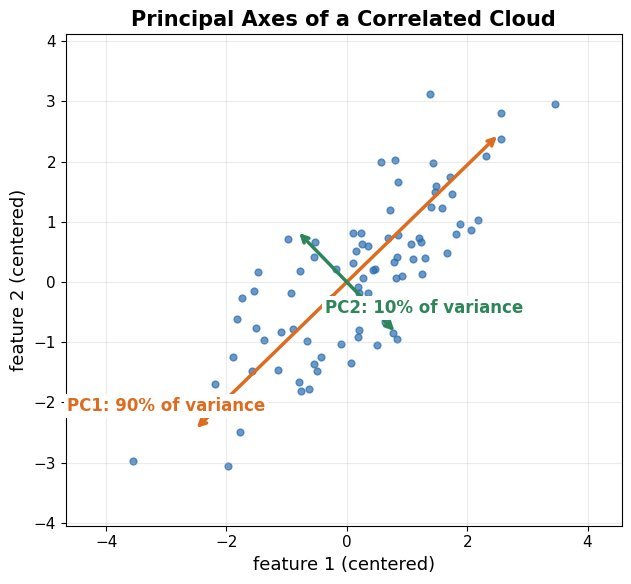
Two-dimensional elliptical point cloud with the first principal component arrow along the major axis and the second along the minor axis

Figure 1: The two principal components of a 2D cloud: PC1 lies along the direction of maximum spread and carries the largest eigenvalue; PC2 is orthogonal to it and mops up the residual variance.

Mathematical Formulation:
$\Sigma = \frac{1}{N} X^{\top} X \ \ (\text{centered } X)$
$\Sigma v_j = \lambda_j v_j$
$z_i = V_k^{\top} x_i$

Where:

$X$ is the centered data matrix with $N$ samples and $d$ features; $\Sigma$ is its $d \times d$ covariance matrix.
$v_j, \lambda_j$ are the eigenvector-eigenvalue pairs of $\Sigma$ , sorted by descending $\lambda_j$ .
$V_k$ stacks the top $k$ eigenvectors and $z_i$ is the $k$ -dimensional score vector of sample $x_i$ .

Scree plot: bars of per-component variance falling off, with a cumulative explained variance line crossing the 95 percent mark

Figure 2: The scree plot: bars show the variance each component carries and the curve shows the cumulative share. Keeping components up to the 95% crossing is the standard rule for choosing $k$ .

Projection is lossy: the discarded components carry the remaining variance, so projecting back into the original space reconstructs the data only up to the kept subspace. In 2D this means every point collapses onto the PC1 line when only one component is kept, which is the geometric picture behind “95% of variance retained”.

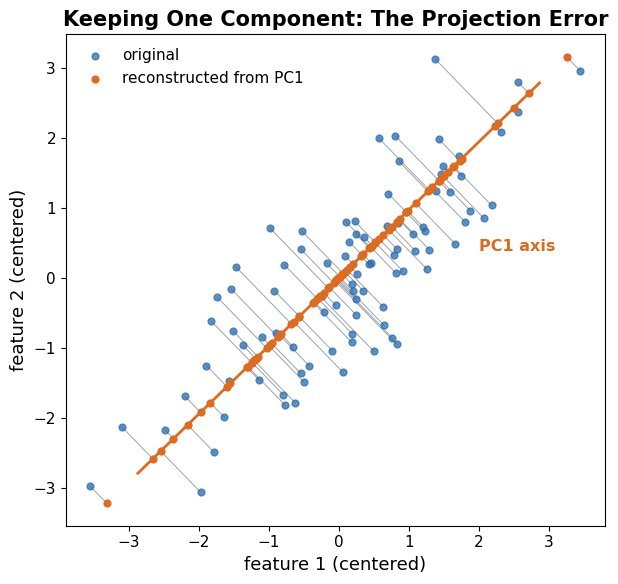
Point cloud with each point connected by a thin line to its perpendicular reconstruction on the principal component axis

Figure 3: Reconstruction from one component: every point is replaced by its perpendicular projection onto the PC1 axis. The gray connectors are the reconstruction errors, whose mean squared length is exactly the discarded variance $\lambda_2$ (their sum is $N \lambda_2$ ).

Feature	Eigendecomposition of Covariance	SVD of the Data Matrix
Input	The $d \times d$ matrix $\Sigma$	The centered $N \times d$ matrix $X$ directly
Numerical Stability	Forming $X^{\top} X$ squares the condition number	Stable: never materializes $X^{\top} X$
Scalability	Fine for small $d$	Randomized SVD scales to huge $N$ and $d$
Practice	Textbook derivation	What libraries (scikit-learn) actually call

August 10, 2026

ML0072 Bayesian Optimization

How does Bayesian optimization (e.g., Gaussian processes) work for hyperparameter tuning, and when is it worth it?

Answer

Bayesian optimization tunes an expensive black-box objective by maintaining a probabilistic surrogate model of it, usually a Gaussian process that predicts both the mean performance and the uncertainty at every untried configuration. An acquisition function (expected improvement is the common default) scores each candidate by trading off exploitation (likely to be good) against exploration (highly uncertain), and the configuration maximizing it is evaluated next; the result updates the surrogate and the loop repeats. It needs far fewer trials than grid or random search when each evaluation costs minutes to hours, but the Gaussian process costs $O(n^3)$ to fit in the number of trials and struggles in high-dimensional or heavily categorical spaces.

(1) Surrogate: the GP posterior gives a predictive mean $\mu(x)$ and uncertainty $\sigma(x)$ from a handful of noisy trials, and it is cheap to query, unlike the real objective.
(2) Acquisition: expected improvement picks the point with the largest expected gain over the incumbent, automatically balancing exploration and exploitation without hand-tuned schedules.
(3) When It Is Worth It: when trials dwarf surrogate cost (minutes or more per trial, tens of dimensions at most). Meta’s Ax platform (built on BoTorch) runs exactly this loop to tune recommender systems and AR/VR hardware designs, while Google’s Vizier has tuned over 70 million objectives and swaps in more scalable algorithms once the trial count outgrows GP fitting costs.

Top panel: Gaussian process posterior mean with a shaded uncertainty band fitted to a few observed points; bottom panel: expected improvement curve peaking at the next point to evaluate

Figure 1: One iteration of the loop: the GP posterior (mean with uncertainty band, top) is fitted to the evaluated points, and the expected-improvement acquisition (bottom) peaks where a high predicted mean and high uncertainty combine. That peak becomes the next expensive evaluation.

Mathematical Formulation:
$\mathrm{EI}(x) = \mathbb{E}\big[\max(f(x) - f^{*}, 0)\big]$
$x_{t+1} = \arg\max_{x}\ \mathrm{EI}(x)$

Where:

$f(x)$ is the expensive black-box objective (for example validation accuracy) and $f^{*}$ the best value observed so far.
The expectation is taken under the GP posterior, so $\mathrm{EI}(x)$ grows both with predicted quality $\mu(x)$ and with uncertainty $\sigma(x)$ .
$x_{t+1}$ is the next configuration to evaluate; the acquisition maximization is cheap because it queries only the surrogate.

Feature	Bayesian Optimization	Grid / Random Search
How Points Are Chosen	Surrogate model plus acquisition function	Fixed lattice / uniform sampling
Trials to a Good Region	Fewest, for smooth low-dimensional objectives	Grows exponentially (grid) or slowly (random)
Per-Step Overhead	GP fit $O(n^3)$ plus acquisition search	None
Parallelism	Needs batch acquisition (qEI)	Trivially parallel
Worth It When	Trials cost minutes or more, up to tens of dimensions	Cheap trials, high dimensions, quick baseline

Best value found so far versus number of evaluations: Bayesian optimization curve rises fastest, random search in the middle, grid search slowest

Figure 2: Best value found so far against evaluations spent. Bayesian optimization’s surrogate-guided choices reach a good region in far fewer trials than random or grid search, which is exactly why it pays off only when each trial is expensive.

August 10, 2026

ML0071 Covariance vs Correlation

What is the difference between covariance and correlation?

Answer

Both measure how two variables move together. Covariance is the raw co-movement, expressed in the product of the two variables’ units: positive when the variables tend to sit above their means together, negative when one runs high while the other runs low. Correlation (Pearson’s $\rho$ ) is covariance divided by both standard deviations, which strips the units and bounds the result to $[-1, 1]$ , so strengths become comparable across datasets. Neither proves causation, and both capture only linear association: a perfect parabola scores zero correlation despite being fully determined.

(1) Units: covariance keeps the product of the units (dollars times kilograms); correlation is unitless and bounded, so rescaling a variable changes the covariance but leaves the correlation untouched.
(2) Sign vs Strength: covariance tells you the direction of co-movement; only correlation tells you a comparable strength, since $0.9$ vs $0.2$ means the same thing for any pair of variables.
(3) Linear Only: both are second-moment statistics of linear association. Zero correlation does not imply independence: $Y = X^2$ on symmetric data has $\rho = 0$ while $X$ fully determines $Y$ .

Four scatter panels: positive correlation, negative correlation, zero correlation with independent points, and a parabola with zero correlation but full dependence

Figure 1: Correlation reads linear co-movement: positive (top left), negative (top right), zero with independence (bottom left), and the trap case, zero correlation with complete dependence on a parabola (bottom right). The first three have matching covariance signs; the fourth shows why a second-moment statistic can miss structure.

Mathematical Formulation:
$\mathrm{Cov}(X, Y) = \mathbb{E}\big[(X - \mu_X)(Y - \mu_Y)\big]$
$\rho_{XY} = \frac{\mathrm{Cov}(X, Y)}{\sigma_X \, \sigma_Y}$

Where:

$X, Y$ are random variables with means $\mu_X, \mu_Y$ and standard deviations $\sigma_X, \sigma_Y$ .
$\mathbb{E}[\cdot]$ is expectation over the joint distribution; in practice both quantities are estimated by sample averages.
$\rho_{XY}$ lies in $[-1, 1]$ by the Cauchy-Schwarz inequality, with $\pm 1$ meaning an exact linear relationship.

Feature	Covariance	Correlation
Definition	Mean product of centered values	Covariance divided by both $\sigma$
Units	Product of the variables’ units	Unitless
Range	Unbounded	$[-1, 1]$
Scale Invariance	No: rescaling a variable rescales it	Yes: unchanged by a positive affine rescaling (a negative scale flips the sign)
Typical Use	Portfolio variance, covariance matrices, PCA	Comparing association strength, feature screening

August 10, 2026

ML0070 A/B Test Design

How would you design an A/B test, including sample size and duration?

Answer

An A/B test is a randomized controlled trial: randomly assign users to control (A) and treatment (B), measure a pre-registered primary metric, and compare the two arms with a hypothesis test. The design happens before any traffic flows: pick one primary metric and a minimum detectable effect (MDE), fix $\alpha$ and power (0.05 and 0.8 are common defaults), and compute the required sample size per arm from the metric’s variance. Duration follows from daily traffic, rounded up to whole business cycles (at least one to two weeks) so day-of-week effects average out, and the decision is made once at the pre-committed end rather than by peeking at daily p-values.

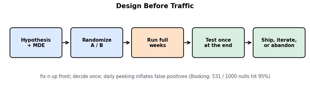
(1) Hypothesis and MDE First: state the expected effect and the smallest effect worth shipping for. The MDE, $\alpha$ , power, and metric variance together pin down the sample size.
(2) Duration by Cycles, Not by Peeking: run whole weeks to cover weekly seasonality and never stop early on a crossing p-value. Booking.com simulated null experiments and found that daily peeking lets over half of them touch 95% significance at some point, versus the promised 5%.
(3) Sensitivity Is the Bottleneck: variance reduction beats longer runs. CUPED (developed at Microsoft) uses pre-experiment covariates to cut metric variance by about 50%, halving the required users or duration, and Booking.com warns that tracking users the change cannot reach dilutes the measured effect and inflates the required sample size by the dilution factor squared.

Flow diagram: hypothesis with MDE leads to random assignment into arms A and B, then a run of full weekly cycles, then one test at the pre-committed end, then a ship or iterate decision

Figure 1: The design pipeline: fix the hypothesis, MDE, $\alpha$ , and power up front; randomize; run whole business cycles; test exactly once at the pre-committed sample size; then ship, iterate, or abandon.

Mathematical Formulation:
$n = \frac{2 \, (z_{1-\alpha/2} + z_{1-\beta})^2 \, \sigma^2}{\delta^2}$
$\sigma^2 = p \, (1 - p) \ \text{for a binary metric}$

Where:

$n$ is the required sample size per arm; $\delta$ is the MDE; $\sigma^2$ is the per-user metric variance.
$z_{1-\alpha/2}$ and $z_{1-\beta}$ are normal quantiles for the significance level and power (1.96 and 0.84 at the usual settings).
$p$ is the baseline rate for a binary metric such as conversion, whose variance is set by $p(1 - p)$ .

Sample size per arm on a log scale falling with the square of the minimum detectable effect, with a marked point at 1 percentage point MDE on a 10 percent baseline needing about 14400 users per arm

Figure 2: Sample size per arm falls with the square of the MDE: halving the detectable effect quadruples the traffic needed. On a 10% conversion baseline, a 1-point MDE needs about 14,400 users per arm; a 0.25-point MDE needs about 230,000.

Decision Rule	When You Look	False Positive Control	Cost
Fixed horizon (pre-committed n)	Once, at the end	Exact $\alpha$	Requires patience
Naive peeking	Daily, stop on significance	Inflated: Booking’s nulls hit 95% over half the time	Ships noise
Sequential test (mSPRT, group-sequential)	Any time	Controlled by construction	Wider confidence sequences

Two histograms of the estimated treatment minus control difference: a wide raw distribution and a narrow CUPED-adjusted distribution centered on the same effect

Figure 3: CUPED regresses out the part of the metric explained by pre-experiment behavior, leaving the same estimated effect with roughly half the variance. That is equivalent to doubling the sample size without adding a single user.

August 10, 2026

ML0069 Z-Test vs T-Test

When do you use a z-test versus a t-test?

Answer

Both tests compare an estimated effect with its standard error to judge whether a mean differs from a reference value. Use a z-test when the reference distribution can be treated as exactly normal: the population standard deviation $\sigma$ is known, or the sample is large enough that the estimate of $\sigma$ is essentially exact. Use a t-test when $\sigma$ is estimated from a small sample: the extra estimation uncertainty fattens the tails of the test statistic, and the t-distribution with $n - 1$ degrees of freedom accounts for it. As $n$ grows, the t-distribution converges to the normal, so beyond a few dozen observations the two tests give nearly identical p-values.

(1) Same Statistic, Different Reference: both divide an effect estimate by its standard error; they differ only in whether the reference distribution is the standard normal or the heavier-tailed t.
(2) When t Is Mandatory: small samples with unknown $\sigma$ , where the t’s heavier tails keep the false positive rate at the promised $\alpha$ . Use Welch’s variant when the two groups have unequal variances.
(3) In Practice at Scale: conversion metrics in online experiments are proportions with millions of users, so the normal (z) approximation is effectively exact; Booking.com’s experimentation write-ups fall back to the two-sample t-test when comparing means on smaller or skewed samples.

Standard normal curve overlaid with a heavy-tailed t distribution with 3 degrees of freedom, the t tails visibly higher beyond plus minus 2

Figure 1: Why the distinction exists: the t-distribution (3 degrees of freedom shown) has visibly heavier tails than the standard normal, so its critical values sit farther out. As degrees of freedom grow, the t curve collapses onto the normal and the two tests coincide.

Mathematical Formulation:
$z = \frac{\bar{x} - \mu_0}{\sigma / \sqrt{n}}$
$t = \frac{\bar{x} - \mu_0}{s / \sqrt{n}}$

Where:

$\bar{x}$ is the sample mean, $\mu_0$ the hypothesized mean, and $n$ the sample size.
$\sigma$ is the known population standard deviation used by the z-test; $s$ is the sample-estimated standard deviation used by the t-test.
The t statistic follows a t-distribution with $n - 1$ degrees of freedom, which approaches $N(0, 1)$ as $n$ grows.

Feature	Z-Test	T-Test
Spread Parameter	$\sigma$ known (or $n$ huge)	$s$ estimated from the sample
Reference Distribution	Standard normal	t with $n - 1$ degrees of freedom
Tail Behavior	Thinner tails, tighter critical values	Heavier tails at small $n$
Typical Case	Proportion tests at scale (conversion)	Small samples, heavy-tailed metrics
Large-n Behavior	Asymptotically valid for proportions via the CLT	Coincides with the z-test

August 10, 2026

ML0068 Type I vs Type II Errors
What are Type I and Type II errors, and how do they trade off?
Answer
A Type I error (false positive) rejects a true null hypothesis: you announce an effect that is not there. A Type II error (false negative) fails to reject a false null: a real effect goes undetected. Their rates are $\alpha$ , the significance level you choose up front, and $\beta$ , with power equal to $1 - \beta$ . For a fixed sample size the two trade off through the decision threshold: making the test stricter lowers $\alpha$ but raises $\beta$ , and only more data or lower metric variance reduces both at once.
(1) Type I ( $\alpha$ ): rejecting a true null, the “convicting the innocent” error. It is controlled by fixing $\alpha$ before looking at data and by correcting when many hypotheses are tested at once.
(2) Type II ( $\beta$ ): missing a real effect. Power $1 - \beta$ grows with sample size, true effect size, and lower metric variance.
(3) Costs Set the Threshold: the right balance is a business decision. Gmail blocks over 99.9% of spam while misrouting only about 0.05% of legitimate mail, because a false positive (lost mail) costs far more than a false negative (spam seen in the inbox).

Figure 1: Sampling distribution of the test statistic under $H_0$ (left) and $H_1$ (right) with one decision threshold. The right tail of $H_0$ is $\alpha$ (Type I), the part of $H_1$ left of the threshold is $\beta$ (Type II), and the rest of $H_1$ is power.
Mathematical Formulation:
$\alpha = \Pr(\text{reject } H_0 \mid H_0 \text{ true})$
$\beta = \Pr(\text{fail to reject } H_0 \mid H_1 \text{ true})$
$\text{power} = 1 - \beta$
Where:
$H_0$ is the null hypothesis (no effect) and $H_1$ the alternative (a real effect exists).
$\alpha$ is the significance level chosen before the test; $\beta$ is the false negative rate under a specific true effect.
Power is the probability of detecting the effect when it is real, and it rises with sample size, effect size, and reduced variance.

Figure 2: Moving the threshold at fixed sample size swaps the errors: stricter (left panel) shrinks $\alpha$ and inflates $\beta$ ; looser (right panel) does the reverse. Shrinking both at once requires more data or lower variance, which pulls the two curves apart.
Decision \ Reality H0 True (No Effect) H1 True (Real Effect)
Reject H0 Type I error, rate $\alpha$ Correct detection, power $1 - \beta$
Fail to Reject H0 Correct, rate $1 - \alpha$ Type II error, rate $\beta$
Login to view more content
August 10, 2026

Decision \ Reality	H0 True (No Effect)	H1 True (Real Effect)
Reject H0	Type I error, rate $\alpha$	Correct detection, power $1 - \beta$
Fail to Reject H0	Correct, rate $1 - \alpha$	Type II error, rate $\beta$

ML0067 Probability vs Likelihood

What is the difference between probability and likelihood?

Answer

Probability and likelihood use the same joint density $p(x \mid \theta)$ but read it in opposite directions. Probability fixes the parameters $\theta$ and asks how plausible different data $x$ are; likelihood fixes the observed data and asks which parameter values would have made that data plausible. A probability distribution must sum or integrate to 1 over all possible data; a likelihood carries no such constraint over the parameters. Maximum likelihood estimation is exactly this direction flip: hold the sample fixed and choose $\theta$ to make the observed data as probable as possible.

(1) Same Formula, Two Directions: with $\theta$ fixed, $p(x \mid \theta)$ is a probability over data; with $x$ fixed at the observed sample, the same expression becomes the likelihood $L(\theta \mid x)$ , a function of $\theta$ .
(2) Normalization: probabilities integrate to 1 over all possible data, while likelihoods do not integrate to 1 over $\theta$ , so a likelihood is never “the probability of the parameter”.
(3) Where Each Is Used: probability drives prediction and simulation of unseen data; likelihood drives parameter estimation. Amazon’s DeepAR forecaster is trained by maximizing the likelihood of observed demand series, then at inference emits probability distributions over future demand.

Two panels: left, a probability density over data values with parameters fixed; right, a likelihood curve over the parameter theta with data fixed, peaking at the maximum likelihood estimate

Figure 1: The same density viewed two ways. With $\theta$ fixed, the curve over data values is a probability distribution and integrates to 1 (left). With the data fixed at the observed sample, the curve over $\theta$ is the likelihood (right), whose peak is the maximum likelihood estimate.

Mathematical Formulation:
$L(\theta \mid x) = p(x \mid \theta)$
$\hat{\theta}_{\mathrm{MLE}} = \arg\max_{\theta}\ \sum_{i=1}^{N} \log p(x_i \mid \theta)$

Where:

$x$ is the observed data and $\theta$ the model parameters.
$p(x \mid \theta)$ is the density of the data under parameters $\theta$ ; $L(\theta \mid x)$ is the same expression read as a function of $\theta$ .
$x_i$ with $i\in\{1,\ldots,N\}$ indexes independent samples, so the joint likelihood factorizes into a product and the logarithm turns it into a sum.

Feature	Probability	Likelihood
What Varies	The data $x$	The parameters $\theta$
What Is Fixed	The parameters $\theta$	The observed data $x$
Normalization	Binomial example: P(X = 3) = C(10,3)0.3^30.7^7 = 0.267	No constraint over $\theta$
Answers	“What data should I expect?”	“Which parameters fit the data I saw?”
Typical Use	Prediction, simulation, p-values	Estimation (MLE), model comparison

August 10, 2026

MSD0017 Meeting Summarization
Design the system behind Zoom AI Companion’s meeting summary: after a 45-minute video meeting, every participant receives a recap, the decisions made, and their action items within a minute or two. The pipeline must handle cross-talk, accents, and bad microphones across ten speakers, and a hallucinated action item is worse than none at all.
How would you design this system? Cover transcription, speaker attribution, the summarization stack, quality control, privacy, and cost at platform scale.

The Problem: forty-five minutes of overlapping speech from ten microphones must become a recap, a decision list, and attributed action items, within minutes, and one invented task destroys trust. Design the pipeline that was actually listening.
Answer
The design is a staged pipeline with a federated summarization stack, the approach Zoom publishes for AI Companion: streaming ASR turns audio into words, speaker diarization attributes them to people, a post-processing stage restores punctuation and domain terms, and the summarization stage drafts on a small in-house LLM, scores the draft with a learned quality model (Zoom’s Z-Scorer), and escalates to a stronger external LLM only when the score is low. The two pivotal decisions are separating “who spoke” from “what was said” (diarization plus ASR reconciled with the meeting roster, not one giant model asked to guess names) and never paying frontier-model prices for meetings a small model summarizes fine (Zoom reports comparable quality at roughly 6% of GPT-4 cost).
(1) ASR Frontend: streaming encoder-decoder (Whisper-class) with custom vocabulary biasing for product and people names; about 95% word accuracy on real meetings.
(2) Speaker Diarization: embedding-based turn detection (pyannote-style) reconciled with the participant roster and per-channel audio when available, so “Speaker 2” becomes “Ada”.
(3) Structured Summarization: chained tasks with schema-checked JSON output: chapter segmentation, recap, decisions, action items with owners.
(4) Federated Quality Control: small model drafts, a learned scorer predicts summary quality, low scores escalate to stronger LLMs, and a committee-of-LLMs cross-check suppresses hallucinated action items.
(5) Privacy by Inheritance: summaries inherit the meeting’s access control and retention; a self-hosted-only model path serves regulated customers.

Figure 1: The pipeline: hear the words, attribute them, then summarize with schema-checked structure; the scorer, not blind trust, decides when a stronger model is worth paying for.
Clarify Before Designing:
(1) Live versus Post: in-meeting “catch me up” queries (seconds, incremental) or post-meeting delivery only (minutes, batch)?
(2) Language Scope: English only, or 30-plus languages via translation assists or multilingual models?
(3) Identity Source: is a participant roster, per-channel audio, or voice enrollment available, or must speakers stay anonymous labels?
(4) Worst Error: which failure is most expensive here: hallucinated action items, missed decisions, or wrong attribution?
(5) Scale and Budget: meetings per day, average length, and the cost ceiling per meeting-minute?
Login to view more content
August 9, 2026
MSD0016 Scanned Document OCR
Design an OCR system that converts millions of scanned documents (contracts, invoices, old books, fax-quality pages) into clean, structured text for a document platform like AWS Textract, Google Document AI, or Mistral’s OCR API. The output must preserve reading order, tables, and equations, not just raw characters, because the text feeds search indexes and RAG pipelines downstream.
How would you design this system? Cover the recognition approach, layout and structure handling, accuracy measurement, and the cost of processing at scale.

The Problem: a skewed, coffee-stained scan of a two-column contract must come out as correctly ordered, structured text, at millions of pages, at a cost a business can pay. Design the reader that never silently scrambles a page.
Answer
The design is a single-pass document VLM pipeline in the style of AI2’s olmOCR: lightweight preprocessing normalizes each page (orientation, deskew, denoise, blank rejection), then a fine-tuned 7B-class vision-language model reads the whole page in one pass and emits structured output (Markdown for headings, HTML for tables, LaTeX for math), and programmatic unit tests verify each page (does the table parse? does the equation recompile? is reading order sane?) before failures are retried or routed to a stronger model or a human queue. The two pivotal decisions are reading whole pages in one pass instead of a detect-then-crop-then-recognize cascade (which accumulates errors and loses reading order), and defining correctness as machine-checkable tests so both evaluation and training optimize what downstream consumers actually need.
(1) Single-Pass VLM Reader: a fine-tuned Qwen2.5-VL-class model turns a page image directly into structured Markdown/HTML/LaTeX, skipping the multi-stage cascade.
(2) Document Anchoring: born-digital PDFs contribute their embedded text and metadata into the prompt alongside the page image, grounding the model and cutting hallucination.
(3) Preprocessing Gate: orientation detection, deskew, denoise, and blank-page rejection run before the expensive model call.
(4) Verifiable QA: per-page unit tests (table parses, math recompiles, reading order monotonic); failures retry with different sampling or escalate to a stronger model or human review.
(5) Batch-First Serving: offline GPU batches with vLLM/SGLang; a tuned open pipeline processes a million pages for roughly $190, about 1/32 of frontier-API pricing.

Figure 1: The pipeline: cheap normalization first, one VLM read per page, then machine-checkable tests decide whether the page ships, retries, or goes to a human.
Clarify Before Designing:
(1) Document Mix: born-digital PDFs versus degraded scans; which languages; is handwriting in scope?
(2) Structure Fidelity: plain text, or RAG-grade structure with tables, equations, and reading order preserved?
(3) Volume and Latency: nightly millions in batch, or interactive upload-and-wait in seconds?
(4) Deployment Constraints: customer data residency or full self-hosting requirements (regulated archives)?
(5) Downstream Contract: does the consumer want Markdown, or structured JSON field extraction (invoice totals, dates) on top?
Login to view more content
August 9, 2026
MSD0015 LLM Request Routing
Design the routing layer for an AI assistant that chooses, per request, between a small cheap model and a large expensive one. ChatGPT’s GPT-5 does exactly this with a real-time router that picks between its fast and reasoning variants, and research frameworks like RouteLLM show a trained router can cut serving cost by over 80% while holding about 95% of the strong model’s quality.
How would you design this system? Cover what the router sees and how it is trained, how answer quality is guarded, the cost accounting, and how the system adapts as models are added, upgraded, or deprecated.

The Problem: most requests are easy, a few are hard, and sending everything to the biggest model burns money on “hello”. Design the gate that sends each request down the cheapest road that still answers it well.
Answer
The design is a trained per-request router: a tiny scorer reads the request and predicts the probability that the strong model’s answer beats the weak one’s, then sends the request to the cheapest model expected to clear the quality bar. This is routing, not cascading, so each request normally pays for exactly one model. The two pivotal decisions are to train the router on human preference data (which model’s answer people actually preferred, as in Chatbot Arena battles) rather than hand-built rules, and to expose an explicit cost-quality operating threshold as a product knob, with an escalation fallback so a routing mistake costs extra compute, not a bad answer.
(1) Difficulty Signals: query embedding and length, task type, tool needs, and conversation state; the router is BERT-class or smaller, ~1/1000 the cost of a strong call.
(2) Preference-Trained Router: learn P(strong model wins | query) from human preference battles, augmented with LLM-judged comparisons; route strong when P passes the threshold.
(3) Explicit Operating Point: the threshold is chosen on the measured cost-quality curve and recalibrated as the traffic mix drifts.
(4) Guarded Fallback: if the small model or a verifier flags low confidence, escalate to the large model; routing errors become cost, not bad answers.
(5) Model Registry & Shadowing: candidates live behind a versioned registry; new models are shadow-scored on live traffic before the router is retrained or recalibrated.

Figure 1: The routing path: one cheap score per request, one paid model call, and an escalation hatch when the cheap path doubts itself.
Clarify Before Designing:
(1) Candidate Set: two models or many; closed APIs, self-hosted weights, or both; is the real split fast-versus-reasoning rather than small-versus-large?
(2) Decision Granularity: per request, per message in a conversation, or pinned per session for style consistency?
(3) Quality Bar: which evaluation defines “good enough” (human preference, task success), and how much loss versus the always-strong policy is tolerable?
(4) Router Budget: how much latency and cost may the router itself add per request?
(5) Traffic Shape: what fraction of traffic is trivial chat versus hard reasoning today, and how fast does that mix drift?
Login to view more content
August 9, 2026