Author: admin

  • MSD0014 Music Identification

    Design a music identification system like Shazam: a user holds up a phone in a noisy cafe, records a 10-second snippet, and the app names the song within a second. Apple’s ShazamKit exposes the same matching to third-party apps, Google’s “Now Playing” identifies music continuously and offline on Pixel phones, and SoundHound even accepts hummed melodies.

    How would you design this system? Cover the audio fingerprint representation, the matching index, the latency and scale budget, and how the system behaves under noise, tempo changes, and remixes.

    Line-art scene: a cafe loudspeaker playing a song, a phone recording a short snippet through noise waves, and a question mark asking which song is playing

    The Problem: ten seconds of music buried in cafe noise must pick one recording out of tens of millions, in under a second, and a wrong answer is worse than none. Design the system that hears the song through the crowd.

    Answer

    The design is audio fingerprinting with landmark hashes, the approach Shazam published in 2003 and which remains the backbone of production matchers: convert audio to a spectrogram, keep only the strongest time-frequency peaks (a constellation map that survives noise), hash pairs of peaks into compact tokens, and match a query by finding reference tracks whose hashes recur with one consistent time offset. The two pivotal decisions are to match a lossy peak representation instead of the waveform (robustness to noise, codec compression, and reverb) and to use an inverted index over hashes with time-coherence voting, which turns “find this song” into a few hundred lookups and a histogram test rather than a comparison against the whole catalog.

    (1) Constellation Frontend: STFT spectrogram, keep local peaks only; noise must out-shout a peak to erase it, so ~20 peaks/second survive a cafe.
    (2) Combinatorial Hashing: each anchor peak pairs with peaks in a short target zone; the hash packs both frequencies and the time gap, giving millions of distinct tokens.
    (3) Inverted Index + Offset Voting: hash to list of (track, time) postings; matching query hashes vote on the offset, and a histogram spike declares the track.
    (4) Asymmetric Confidence: naming the wrong song costs more than “no match found”, so an answer needs enough aligned votes plus a margin over the runner-up.
    (5) Catalog Ingestion at Scale: new releases are fingerprinted as labels deliver them; the index is sharded by hash and held in RAM for sub-second queries.

    Music identification pipeline: a register lane fingerprints catalog tracks into a hash index, and a recognize lane turns a noisy snippet into hashes, votes on time offsets, and returns the track title

    Figure 1: Register and recognize lanes share one fingerprinting frontend; recognition is index lookups plus offset voting, never a comparison against raw audio.

    Clarify Before Designing:
    (1) Query Conditions: phone microphone in noise versus clean line-in audio, and how short a snippet must work (5 s? 15 s?)?
    (2) Catalog Scope: tens of millions of commercial tracks, and do covers, remixes, and live versions count as the same song?
    (3) Latency Budget: sub-second answer on a mobile connection, or is a few seconds acceptable?
    (4) On-Device versus Cloud: must matching run offline with a regional catalog subset (the Now Playing design), or is the phone always online?
    (5) Beyond Exact Recordings: is humming or cover identification in scope (a different, melody-based representation), or exact audio only?


    Login to view more content
  • MSD0013 Machine Translation at Scale

    Design a machine translation system for a product like Google Translate: text translation between 100+ language pairs, from high-resource pairs like English-Spanish down to low-resource languages with little parallel data, served interactively at web scale where users expect answers in a fraction of a second.

    How would you design this system? Cover the model architecture, how you get training data for low-resource languages, the serving design, and how you measure translation quality.

    Line-art scene: a grid of language nodes with dense cross edges illustrating the quadratic language-pair explosion, one document flowing in and translated copies flowing out, and a question mark over how to cover low-resource pairs

    The Problem: 100 languages mean roughly 10,000 directed pairs, most with almost no parallel data, and users still expect every pair to answer in milliseconds. Design one system that covers them all.

    Answer

    The design is a single massively multilingual encoder-decoder model trained on mined bitext plus back-translated monolingual text, with a target-language token steering generation (the NLLB recipe), behind a dual-track serving layer: a fast NMT track for short, latency-critical, terminology-sensitive text, and a fine-tuned translation LLM for long, nuanced, document-level input, which is exactly the split Google shipped in its Cloud Translation API (2024) and DeepL shipped as its next-gen model. The two pivotal decisions are the multilingual pooling (high-resource pairs teach low-resource ones through a shared representation, enabling zero-shot pairs) and the honest admission that one model family does not win everywhere: NMT still wins on latency, cost, and determinism, the LLM wins on context and fluency.

    (1) One Multilingual Model: shared encoder-decoder with a target-language token; transfer from high-resource pairs gives zero-shot coverage of unseen pairs instead of 10,000 separate models.
    (2) Data Flywheel: mine bitext from web crawls with multilingual sentence embeddings (LASER), then back-translate monolingual text to synthesize pairs for low-resource languages.
    (3) Dual-Track Serving: NMT for short/interactive/terminology-critical requests, translation LLM for long-form and idiomatic text; a router picks per request.
    (4) Quality Measurement: automatic metrics (COMET, BLEU) for regression, human MQM error marking for truth, A/B tests for product impact, all reported per language pair.
    (5) Low-Resource Strategy: zero-shot transfer first, then few-example adaptive conditioning (Google’s Adaptive Translation shows as few as 5, and up to 30k, example pairs can steer output at inference time).

    Translation architecture: source text enters a router that sends short interactive text to a fast NMT track and long nuanced text to a translation LLM track, both share multilingual training on mined bitext and back-translation, and outputs pass terminology constraints before serving

    Figure 1: Dual-track serving over one multilingual training base: the router sends short, latency-critical text to NMT and long, context-heavy text to the translation LLM; terminology constraints apply on both tracks.

    Clarify Before Designing:
    (1) Scope: text only, or also speech and image translation; and which language pairs at launch?
    (2) Latency Budget: interactive typing (sub-300 ms) versus document translation (seconds) imply different model families.
    (3) Quality Bar: gist-level understanding for users, or publication-grade output with human post-editing?
    (4) Terminology: must product names, legal terms, or brand glossaries be honored exactly?
    (5) Customization: do enterprise customers need domain adaptation (medical, legal) with their own example pairs?


    Login to view more content
  • MSD0012 Wake-Word Detection

    Design a wake-word detection system (e.g., Amazon’s “Alexa” or Apple’s “Hey Siri”) that spots a trigger phrase in a continuous audio stream on a phone or smart speaker. It must listen always-on without draining the battery, wake almost instantly when the user speaks, and almost never fire by mistake.

    How would you design this system? Cover the on-device architecture, the detection model, the training data, and how you measure accuracy.

    Line-art scene: a continuous audio waveform flowing into a smart speaker, one segment highlighted as the trigger phrase, a battery icon with a tight power budget, and a question mark over false alarms versus missed triggers

    The Problem: the detector discards nearly 100% of everything it hears, yet the one time it must fire, it has milliseconds and milliwatts to decide. Design the system that never sleeps but barely sips power.

    Answer

    The design is a two-stage cascade split across processors, the architecture Apple describes for its voice trigger system: a tiny streaming detector runs on the always-on low-power processor (DSP/AOP) tuned for high recall, and when it fires, a buffered audio segment goes to a larger, high-precision checker on the main application processor, optionally followed by speaker verification so only the enrolled user wakes the device. The two pivotal decisions are the cascade itself (the power budget makes one big always-on model impossible) and the operating point: false accepts are counted per unit of listening time (research reports them per hour of audio, products budget them per device-day) and they dominate the cost, so thresholds are tuned on an FA-versus-miss curve, not on accuracy.

    (1) Cascade Across Processors: stage 1 is a tiny quantized DNN on the always-on processor (high recall, permissive); stage 2 is a larger checker on the application processor (high precision) fed from a ring buffer.
    (2) Streaming Frontend: 16 kHz audio, 10 ms hops, log-mel filterbank frames, DNN posteriors over sub-word states, and a temporal integrator (HMM-style) that turns frame scores into one detection score.
    (3) Asymmetric Objective: false accepts per device-day is the headline metric; a second-chance threshold band briefly raises sensitivity after a near-miss instead of paying FA cost all the time.
    (4) Data Engine: real trigger recordings plus TTS-synthesized ones, augmented with noise, reverb, and far-field impulse responses, plus hard negatives (e.g., “seriously” for “Hey Siri”).
    (5) Privacy by Construction: no audio leaves the device before activation; personalization (speaker ID) runs on-device after enrollment.

    Wake-word cascade: microphone feeds a frontend and a tiny stage-one detector on the always-on processor, a ring buffer hands candidate audio to a larger stage-two checker on the application processor, then speaker verification, then the assistant activates

    Figure 1: The cascade: a high-recall listener on the low-power chip gates a high-precision checker on the main chip; a ring buffer carries the candidate audio across so no trigger onset is lost.

    Clarify Before Designing:
    (1) Device Class: phone, watch, or smart speaker; battery and DSP availability decide stage sizes (a watch gets ~5% of a tiny compute budget).
    (2) Trigger Spec: one phrase or several, fixed phrase or user-custom, and must it work hands-free in far-field rooms?
    (3) False-Accept Budget: how many accidental activations per day are tolerable, and what do they cost (battery, privacy review, user trust)?
    (4) Personalization: should only the enrolled owner’s voice trigger it, or anyone’s?
    (5) Cloud Role: may a cloud verifier re-check activations, or is the device fully offline?


    Login to view more content
  • MSD0011 LLM Evaluation Pipeline

    Your team ships an LLM-powered product: a customer-support copilot built on a foundation model API, similar in spirit to how GitHub evaluates models for Copilot before each release. The model version, prompts, retrieval index, and tools all change every few weeks, and every change can silently alter answer quality.

    Design an evaluation pipeline that runs before each release. What do you test, how do you score open-ended outputs, and how do you decide whether the new version is safe to ship?

    Line-art scene: a release train carrying a new model version and new prompts toward a production gate, a clipboard with quality metrics, and a question mark over whether the new version regressed

    The Problem: the system under test is stochastic, so a green build means nothing without a repeatable quality signal. Design the gate between “we changed the prompt” and “customers see it.”

    Answer

    The design is a CI pipeline for a stochastic system: a curated golden suite mined from real production failures, a grader ladder (deterministic checks where possible, an LLM judge calibrated against human labels where necessary, human audits on top), and a release gate that compares the candidate against the current version on quality metrics plus guardrails (safety, latency, cost). GitHub runs more than 4,000 such offline tests in CI before any Copilot model change; Anthropic’s guidance is to start with 20 to 50 tasks drawn from real failures and grow from there. The pipeline ends in a canary and A/B test, and production monitoring feeds new failures back into the suite, so the eval set is a living artifact.

    (1) Cases From Reality: the golden suite is mined from production logs, bug reports, and support tickets, not invented at a desk; 20-50 real tasks beat 500 synthetic ones.
    (2) Grader Ladder: deterministic checks first, an LLM judge (calibrated to human labels, pairwise where possible) second, human audits as the calibration anchor.
    (3) Capability vs Regression Suites: capability evals start at a low pass rate and measure progress; regression evals sit near 100% and block backsliding; saturated capability cases graduate into the regression suite.
    (4) Release Gate With Guardrails: the candidate must beat or tie the incumbent on quality with statistical significance, and must not breach guardrails on safety, latency, and cost.
    (5) Flywheel: production failures are mined, de-identified, and converted into new eval cases every release cycle.

    Release evaluation pipeline: a candidate version flows through the golden suite, deterministic checks and an LLM judge with human calibration, a release gate comparing deltas and guardrails, then canary and A/B rollout, with a loop from production logs back into the golden suite

    Figure 1: The pre-release path: golden suite, grader ladder, gate, then canary. The loop back from production logs is what keeps the suite honest as user behavior shifts.

    Clarify Before Designing:
    (1) Product Surface: single-turn answers, multi-turn chat, or an agent with tool calls; the grader design differs sharply.
    (2) What Changes per Release: model version, prompts, retrieval data, tools; each change type needs its own regression coverage.
    (3) Failure Cost: what is the worst plausible wrong answer (refund mistakes, medical tone, leaked PII) and who is accountable for it?
    (4) Human Label Budget: how many expert labels per cycle can we afford, since they anchor the judge’s calibration?
    (5) Release Cadence: weekly prompt tweaks and quarterly model upgrades imply different gate depths.


    Login to view more content
  • MSD0010 Grammar Checking Writing Assistant


    You are building a writing-assistance product like Grammarly. As a user types in a browser extension, email client, or mobile keyboard, the system underlines mistakes and offers corrections in near real time: spelling, punctuation, subject-verb agreement, tense, and for premium tiers, style and clarity rewrites.

    How would you design this system? Cover the model architecture, the latency budget, the training data, and how you evaluate suggestion quality.

    Line-art scene: a document page with several sentences, wavy underlines beneath a misspelled word and a grammar error, a blinking caret mid-sentence, a stopwatch annotated with a 100 ms budget, and a question mark over which model answers fast enough

    The Problem: suggestions must arrive faster than the next keystroke, and a wrong correction costs more trust than a missed error. Design the system behind the wavy underline.

    Answer

    The design is a model ladder behind a per-sentence router: cheap deterministic rules and dictionaries catch spelling and punctuation on-device, an edit-tagging Transformer (one parallel pass over the tokens emitting KEEP, DELETE, INSERT, REPLACE tags) handles most grammatical error correction in the cloud, a seq2seq model takes the sentences that need reordering, and an LLM serves style and clarity rewrites only on demand. The two pivotal decisions are routing each sentence to the cheapest model that can fix it (latency is a product feature), and tuning every error type to a precision-first operating point because false corrections erode trust faster than misses.

    (1) Error Taxonomy Drives Architecture: mechanical errors (spelling, punctuation, agreement) and open-ended style rewrites are different problems and deserve different models.
    (2) Model Ladder With Routing: rules → edit-tagger → seq2seq GEC → LLM, cheapest first; the router reads error type, confidence, and latency budget.
    (3) Precision-First Operating Points: per-error-type thresholds tuned on F0.5, since a wrong correction damages trust more than a miss.
    (4) Latency Engineering: score only the current sentence, cache unchanged text, and keep the inline path under 100 ms end to end.
    (5) Personalization & Dialect: locale (US/UK), register (casual vs formal), and per-user dismiss history modulate which suggestions fire.

    Real-time suggestion pipeline: keystrokes enter a sentence buffer with cache, a router sends the sentence to spell and rules, an edit-tagging model, a seq2seq corrector, or an async LLM, and a suggestion merger renders underlines in the editor

    Figure 1: The inline path: each finished sentence is routed to the cheapest sufficient model, and a merger dedupes overlapping suggestions before rendering underlines. Unchanged text is served from cache.

    Clarify Before Designing:
    (1) Scope: which languages and locales, and is style or clarity rewriting in scope or only mechanical correctness?
    (2) Latency Budget: how many milliseconds for inline suggestions, and is there an async path for long-form checks?
    (3) Deployment: what runs on-device versus in the cloud, given browser-extension and mobile constraints?
    (4) Privacy: may user text leave the device, and are there regulated contexts (legal, medical) to special-case?
    (5) Personalization: can we learn from per-user accept and dismiss behavior, and where may that profile live?


    Login to view more content
  • MSD0009 Restaurant Recommendation System for Food Delivery


    You are building the restaurant recommendation system for a food-delivery platform like Uber Eats or DoorDash. When a user opens the app, the home feed must rank nearby restaurants in a way that converts to orders, while respecting hard logistics: the restaurant must be open, inside the delivery radius, and able to deliver on time given the current courier supply.

    How would you design this system? Cover the retrieval and ranking architecture, the features and objectives, and how you handle cold start for new restaurants.

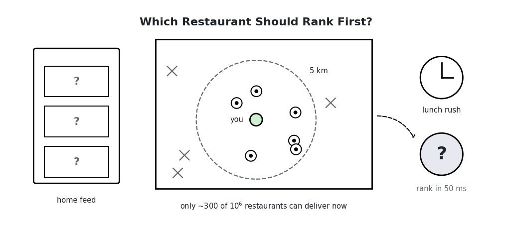
    Line-art scene: a phone showing a restaurant feed stands next to a city map dotted with restaurant pins inside a 5 km delivery circle, a clock marks the lunch rush, and a question mark hangs over which restaurant should rank first

    The Problem: a million restaurants platform-wide, but only a few hundred can actually deliver to this user right now. Rank the right ones first, inside a lunch-rush latency budget.

    Answer

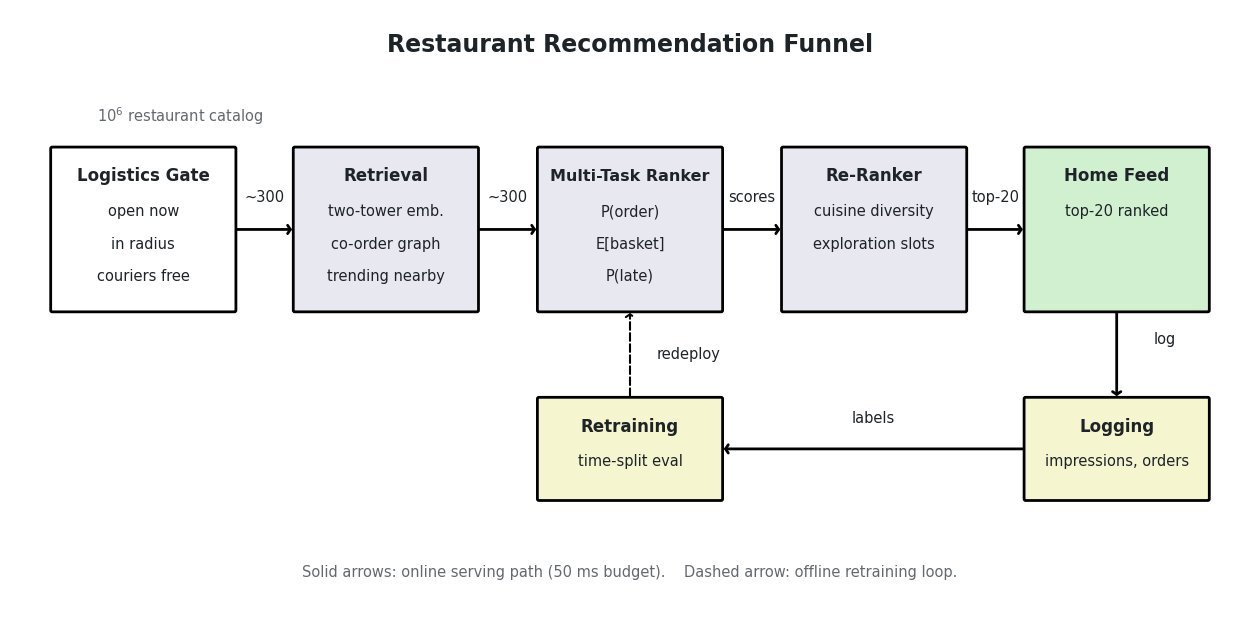
    The design is a multi-stage funnel with a hard logistics gate in front: a geo/open/ETA filter cuts the catalog to the few hundred restaurants that can actually serve the request, multi-source retrieval (two-tower embeddings, co-order graphs, trending-nearby) proposes candidates, a multi-task ranker scores them for order probability, basket value, and delivery time, and a re-ranker enforces cuisine diversity and new-restaurant exploration. The two decisions that make or break the system are treating deliverability as a constraint rather than a feature, and reserving exploration slots so new restaurants ever get seen.

    (1) Funnel, Not One Model: filter → retrieve → rank → re-rank, so each stage stays cheap enough for the 50 ms feed budget.
    (2) Logistics As Hard Filters: open hours, delivery radius, courier supply, and predicted ETA gate eligibility before any learned model runs.
    (3) Context-Heavy Features: time of day, day of week, weather, and session activity matter as much as long-term taste, because lunch intent differs completely from late-night intent.
    (4) Multi-Objective Ranking: combine P(order), expected basket value, and delivery-time risk into one score with explicit business weights.
    (5) Cold Start By Construction: content-based embeddings give new restaurants a Day-1 representation, and reserved exploration slots guarantee them impressions.

    Recommendation funnel pipeline: catalog enters a geo open ETA filter, then multi-source candidate retrieval, then a multi-task ranker, then a re-ranker for diversity and exploration, producing the home feed, with a logging and retraining loop feeding back

    Figure 1: The serving funnel: about one million restaurants shrink to roughly 300 deliverable candidates, then to a ranked top-20 feed. The dashed loop is the offline retraining path fed by logged impressions and orders.

    Clarify Before Designing:
    (1) Scale: how many cities, restaurants, and daily active users, and what is the peak feed QPS at lunch?
    (2) Latency Budget: how many milliseconds for the home feed, and are personalized search results in scope too?
    (3) Objective Priority: is the north star order conversion, gross merchandise value, or delivery-time reliability?
    (4) Cold-Start Volume: how many new restaurants onboard per week, and in how many cities?
    (5) Constraints: must we support sponsored slots, dietary filters, and per-market regulations?


    Login to view more content
  • MSD0008 Cancer Cell Segmentation for Digital Pathology


    A digital pathology lab scans tissue biopsies into gigapixel whole-slide images (WSI). Pathologists currently hunt for tumor regions by panning and zooming across each slide by eye, which is slow and error-prone, and the lab wants software that highlights regions containing cancer cells for priority review.

    How would you design an image segmentation model that detects cancer cells in these slides? Outline the candidate approaches, and explain how you would choose between them.

    Line-art scene: a microscope slide with a tissue region flows into a question mark, a magnifier circle shows hundreds of regular round cells with a few large irregular cancer cells among them, annotated with 100000 by 100000 pixels and about 1 percent cancer pixels

    The Problem: a 100,000 × 100,000-pixel slide, and the cancer signal hides in a tiny fraction of its pixels. Design the segmentation model that fills the question mark.

    Answer

    The task is pixel-level binary segmentation on gigapixel slides: the model labels every pixel as cancer or non-cancer, and the slide is processed as a grid of patches because no GPU holds 1010 pixels at once. Three architecture families cover the realistic design space: the U-Net family (encoder-decoder with skip connections), the DeepLab family (atrous convolutions for wide context at full resolution), and Transformer segmenters (SegFormer-style global context). The choice turns on annotation budget, the spatial context the diagnosis needs, and per-slide compute; a strong default is a U-Net variant trained with an overlap-aware loss under heavy stain augmentation.

    (1) U-Net Family: an encoder compresses each patch, a decoder upsamples back to full resolution, and skip connections re-inject fine detail so cell boundaries stay sharp; the data-efficient default.
    (2) DeepLab / Atrous Family: atrous (dilated) convolutions and ASPP widen the receptive field without shrinking resolution, trading compute for gland-level context.
    (3) Transformer Segmenters: self-attention (SegFormer, TransUNet) models long-range tissue architecture, at the price of a much larger appetite for labeled data or pretraining.

    Encoder-decoder segmentation mechanism: a 256 by 256 tissue patch enters a downsampling encoder staircase and an upsampling decoder staircase with dashed skip connections carrying detail across, producing a same-size cancer mask

    Figure 1: The U-Net mechanism on one patch: the encoder gathers context as it downsamples, the decoder rebuilds the full-resolution mask, and skip connections carry boundary detail straight across. Every 256 × 256 patch yields a same-size cancer mask.

    Clarify Before Designing:
    (1) Imaging Spec: magnification (20× or 40×), typical slide dimensions, and which scanner models feed the pipeline?
    (2) Labels: how many slides carry pixel-level pathologist annotations, and are they full masks, outlines, or only slide-level diagnoses?
    (3) Domain Spread: how many labs, staining protocols, and organ types must one model cover?
    (4) Turnaround Budget: how many minutes per slide may inference take, and on what hardware?
    (5) Cost Asymmetry: a missed tumor region versus a false highlight: which error angers pathologists more?


    Login to view more content
  • DL0067 BERT VS GPT Pretraining

    How does BERT’s pre-training objective differ from GPT’s?

    Answer

    BERT is trained primarily with masked language modeling: selected input tokens are corrupted, and a bidirectional encoder predicts the original tokens from visible context on both sides. GPT uses causal language modeling: a decoder predicts each next token using only earlier tokens, enforced by a triangular attention mask. MLM supplies loss only at selected positions and creates a corruption mismatch between pre-training and ordinary inputs, whereas causal modeling supplies a target at nearly every position and matches left-to-right generation. Original BERT also used next sentence prediction, while standard GPT pre-training relies on the autoregressive token objective rather than NSP.

    (1) Context Visibility: BERT’s visible tokens attend bidirectionally; GPT position t cannot attend to positions later than t.
    (2) Prediction Targets: BERT reconstructs a selected masked subset, while GPT shifts the sequence and predicts the next token at each usable position.
    (3) Downstream Bias: BERT naturally supports full-context understanding, whereas GPT’s objective directly trains open-ended autoregressive generation; either family can be adapted beyond that bias.

    Side-by-side BERT masked-language-modeling and GPT causal-language-modeling pre-training objectives.

    Figure 1: BERT reconstructs selected corrupted tokens from two-sided context, while GPT predicts the next token at every step from a left-only prefix.

    Mathematical Formulation:
    \mathcal{L}_{\mathrm{BERT}}=-\sum_{i\in\mathcal{M}}\log p(x_i\mid x_{\setminus\mathcal{M}})
    \mathcal{L}_{\mathrm{GPT}}=-\sum_{t=1}^{T}\log p(x_t\mid x_{1:t-1})

    Where:

    • \mathcal{L}_{\mathrm{BERT}} and \mathcal{L}_{\mathrm{GPT}} are the masked and causal language-modeling losses.
    • \mathcal{M} is BERT’s selected target set and i\in\mathcal{M} indexes one target token x_i.
    • x_{\setminus\mathcal{M}} denotes BERT’s visible corrupted context outside the selected targets, and p(x_i\mid x_{\setminus\mathcal{M}}) is the reconstruction probability.
    • t\in\{1,\ldots,T\} indexes a GPT target position, T is sequence length, and x_{1:t-1} is the preceding token prefix.
    • p(x_t\mid x_{1:t-1}) is the next-token probability and \log converts each probability into a log-likelihood term.
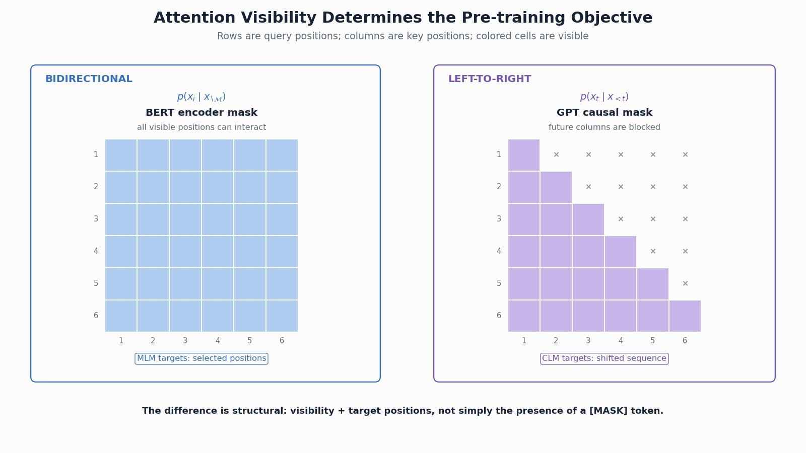
    BERT bidirectional and GPT causal attention matrices with their respective training target positions.

    Figure 2: Attention visibility explains the objective difference: BERT uses a full visible-context matrix, while GPT uses a lower-triangular causal matrix.


    Login to view more content
  • DL0066 BERT

    What is BERT and how is it used in NLP tasks?

    Answer

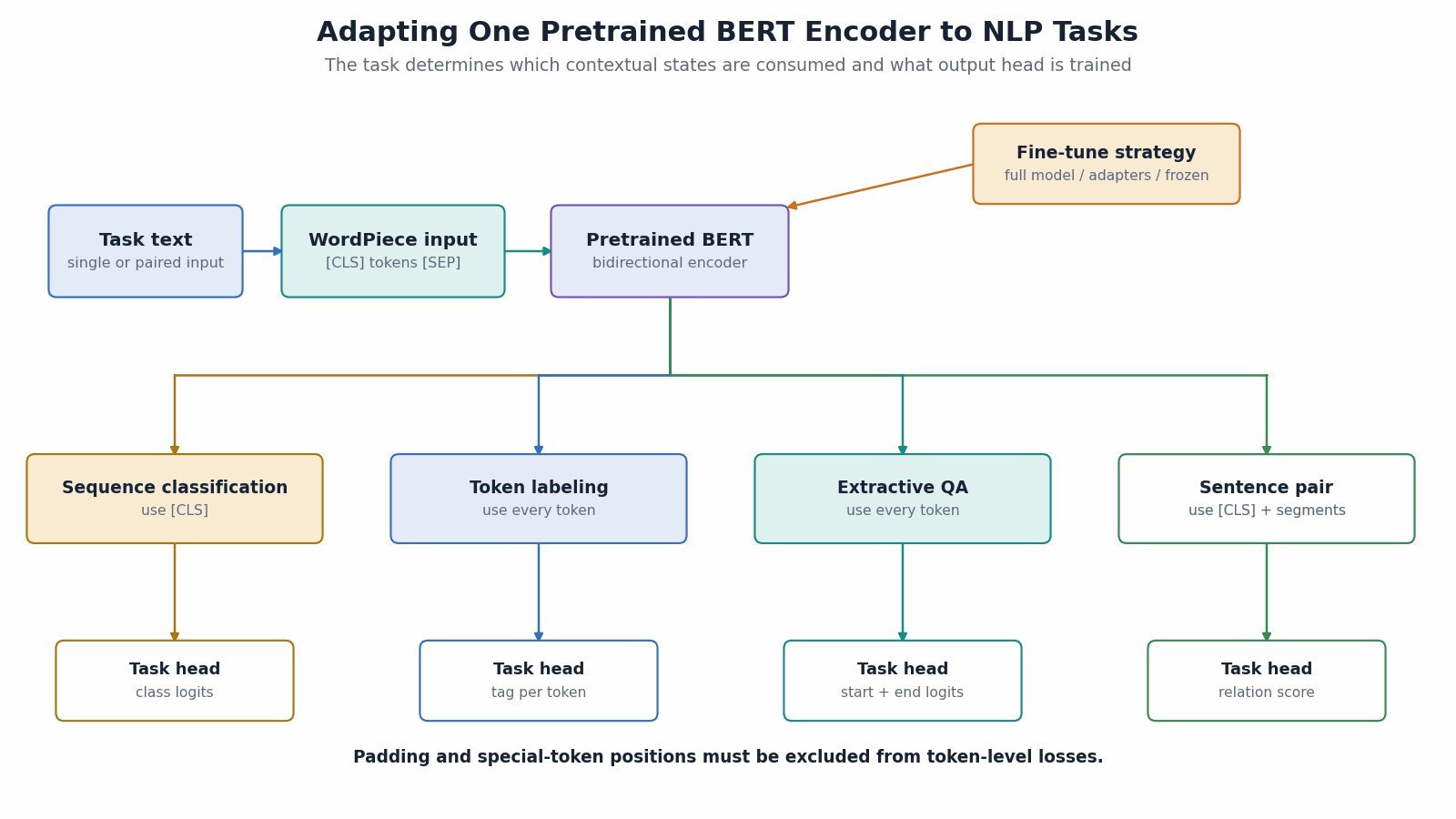
    BERT is a Transformer encoder pretrained to build bidirectional contextual representations of text. Its input combines token, segment, and positional embeddings, and every encoder layer lets each unmasked token attend to context on both sides. Original BERT is pretrained with masked language modeling and next sentence prediction, then adapted by adding a small task head and fine-tuning the whole model or using its representations. The [CLS] output supports sequence-level tasks, token outputs support tagging, and paired start/end scores support extractive question answering.

    (1) Bidirectional Encoder: Unlike a causal decoder, BERT‘s self-attention normally uses both left and right context for every visible input token.
    (2) Pre-Training: Original BERT predicts selected masked tokens and also trains an NSP classifier; later BERT-family models often modify or remove NSP.
    (3) Task Adaptation: A lightweight output head maps contextual states to sequence labels, token labels, sentence-pair scores, or answer spans.

    BERT input embeddings and bidirectional Transformer encoder producing contextual token representations.

    Figure 1: BERT combines token, segment, and position embeddings, processes them with bidirectional encoder layers, and exposes contextual outputs.

    Mathematical Formulation:
    H=\mathrm{Encoder}(E_{\mathrm{token}}+E_{\mathrm{segment}}+E_{\mathrm{position}})
    \mathcal{L}_{\mathrm{MLM}}=-\sum_{i\in\mathcal{M}}\log p(x_i\mid x_{\setminus\mathcal{M}})

    Where:

    • E_{\mathrm{token}}, E_{\mathrm{segment}}, and E_{\mathrm{position}} are token, segment, and positional embedding matrices for the input sequence.
    • \mathrm{Encoder} is the bidirectional Transformer stack and H contains one contextual vector per input position.
    • \mathcal{L}_{\mathrm{MLM}} is masked-language-modeling loss and \mathcal{M} is the selected set of prediction positions.
    • i\in\mathcal{M} indexes one selected target, x_i is its original token, and x_{\setminus\mathcal{M}} denotes the visible corrupted context outside the selected targets.
    • p(x_i\mid x_{\setminus\mathcal{M}}) is the model probability assigned to the original target token given visible context.
    BERT fine-tuning flowchart for classification, token labeling, question answering, and sentence pairs.

    Figure 2: The same pretrained encoder can be adapted with small heads that consume either [CLS], every token state, or start/end span scores.


    Login to view more content
  • DL0065 Group Normalization

    What is Group Normalization?

    Answer

    Group Normalization normalizes each sample independently by dividing its channels into groups and computing a mean and variance over the channels and spatial positions within each group. The normalized activations then receive learned per-channel scale and shift parameters. Because its statistics do not depend on other examples, GroupNorm behaves consistently with very small or variable batch sizes and uses the same computation during training and inference. The group count must be compatible with the channel count, and its inductive bias can be less suitable than BatchNorm when large, stable batches provide useful batch statistics.

    (1) Per-Sample Statistics: Each example has its own group means and variances, so no running batch averages are required.
    (2) Channel Grouping: For C channels and G groups, each group normalizes (C/G)\times H\times W values; channels within a group share statistics.
    (3) Boundary Cases: G=1 normalizes all channels and spatial positions together, while G=C gives one channel per group and resembles InstanceNorm.

    Group Normalization mechanism partitioning channels and normalizing each sample group.

    Figure 1: A convolutional tensor is split into channel groups; each sample-group gets independent statistics before per-channel affine scaling.

    Mathematical Formulation:
    \mu_{n,g}=\frac{1}{m}\sum_{i\in S_{n,g}}x_i
    \sigma^2_{n,g}=\frac{1}{m}\sum_{i\in S_{n,g}}(x_i-\mu_{n,g})^2
    y_{n,c,h,w}=\gamma_c\frac{x_{n,c,h,w}-\mu_{n,g(c)}}{\sqrt{\sigma^2_{n,g(c)}+\epsilon}}+\beta_c

    Where:

    • n indexes samples, g indexes channel groups, and c,h,w index channel and spatial position.
    • S_{n,g} is the set of activations in group g of sample n; i indexes elements in that set.
    • m=(C/G)HW is the number of normalized values when C channels are divided into G groups over height H and width W.
    • \mu_{n,g} and \sigma^2_{n,g} are the group mean and variance; x and y are input and normalized output activations.
    • g(c) maps channel c to its group, \gamma_c,\beta_c are learned per-channel scale and shift, and \epsilon stabilizes division.
    Comparison of Batch, Layer, Instance, and Group Normalization reduction dimensions.

    Figure 2: Normalization families differ mainly in which batch, channel, and spatial axes share statistics and whether inference needs running estimates.


    Login to view more content