Author: admin

  • DL0054 Deformable Attention

    What is Deformable Attention and how does it reduce computational complexity for object detection tasks?

    Answer

    Deformable Attention is a sparse attention mechanism that learns dynamic sampling locations instead of attending to all spatial positions uniformly. It uses learned 2D offsets from reference points to sample only the most relevant features, reducing complexity from O(N^2) to O(NK) where K is a small constant (typically 4). This makes it ideal for high-resolution feature maps in object detection where full attention is computationally prohibitive — for a 1024×1024 feature map (N \approx 10^6 positions), standard attention requires ~1T operations per head while deformable attention needs only ~4M.

    (1) Sparse Sampling: Instead of computing attention over all N \times N positions, deformable attention samples only K reference points per query, typically K=4 or 8, reducing the key-value set from N to K.
    (2) Learned Offsets: The model predicts \Delta p_{mk} offsets from each reference point p_k using a lightweight linear layer on query features, requiring only O(NC) additional computation where C is channel dimension.
    (3) Bilinear Interpolation: When offsets point to non-integer locations, bilinear interpolation computes feature values from the 4 nearest pixels, enabling sub-pixel precision sampling without modifying the feature map.
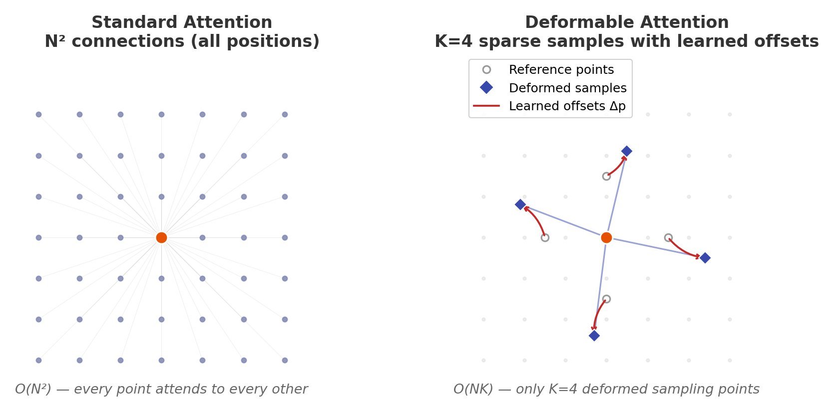
    Sparse Sampling Locations Diagram

    Figure 1: Deformable attention learns K=4 sampling offsets per query point instead of dense N×N attention

    Mathematical Formulation:
    y(p) = \sum_{m=1}^{M} W_m \left[ \sum_{k=1}^{K} A_{mk} \cdot W_m' x(p + p_k + \Delta p_{mk}) \right]

    Where:

    •  p is the reference position (query location on the feature map)
    •  M is the number of attention heads
    •  K is the number of sampled keys per head (typically 4)
    •  p_k are fixed reference offsets (uniformly initialized)
    •  \Delta p_{mk} are learned deformable offsets (2D, predicted per head per key)
    •  A_{mk} is the attention weight (normalized, not from softmax over all positions)
    •  W_m, W_m' are projection matrices for each head
    Complexity Comparison Chart

    Figure 2: Complexity comparison shows O(NK) grows linearly while O(N²) becomes prohibitive for large feature maps

    The offsets \Delta p_{mk} are predicted by a linear projection from query features: \Delta p_{mk} = W_\text{offset} \cdot q_m(p), where W_\text{offset} \in \mathbb{R}^{C \times 2K}. The attention weights A_{mk} are computed via a separate softmax over only K elements, not the full N positions. In Deformable DETR, multi-scale deformable attention extends this to sample across multiple feature map resolutions simultaneously, enabling the model to capture both small and large objects efficiently.


    Login to view more content
  • DL0053 Gated Attention

    What is Gated Attention and how does it improve transformer architectures over standard scaled dot-product attention?

    Answer

    Gated Attention (arXiv:2505.06708) applies a head-specific sigmoid gate after Scaled Dot-Product Attention (SDPA) to dynamically modulate attention output. Unlike standard attention where all heads contribute equally, gated attention introduces query-dependent sparse gating that suppresses irrelevant heads and activates only salient ones. This mitigates the attention sink problem where standard transformers concentrate disproportionate attention on the first few tokens, and enhances long-context extrapolation by maintaining diverse attention patterns across sequence lengths.

    (1) Post-SDPA Gating: The gate is applied after SDPA computation, not before — each attention head h_i is multiplied by a sigmoid gate g_i = \sigma(W_g \cdot q_i) where W_g is a head-specific projection.
    (2) Sparsity Induction: The sigmoid gate produces values in [0, 1], and empirical measurements show mean gate activation of ~0.116, meaning most heads are heavily suppressed — introducing beneficial sparsity without hard pruning.
    (3) Attention Sink Mitigation: Standard attention allocates ~46.7% of attention mass to the first token; gated attention reduces this to ~4.8%, distributing attention more uniformly across tokens.

    Gated Attention Mechanism Diagram

    Figure 1: Gated attention applies a head-specific sigmoid gate after SDPA to modulate attention output before the residual connection

    Mathematical Formulation:
    \text{GatedAttn}(Q, K, V) = \text{Concat}(g_1 \odot h_1, \ldots, g_H \odot h_H) W_O
    g_i = \sigma(W_g^{(i)} \cdot q_i + b_g^{(i)})

    Where:

    •  h_i = \text{SDPA}(q_i, k_i, v_i) is the output of the i-th attention head
    •  g_i \in [0, 1] is the head-specific gate score
    •  W_g^{(i)} \in \mathbb{R}^{d_k \times 1} is a learned projection from query to scalar gate
    •  \sigma is the sigmoid function
    •  \odot denotes element-wise multiplication
    •  W_O is the standard output projection
    Gate Activation Distribution

    Figure 2: Gate activation distribution across 8 attention heads shows heavy suppression (mean ~0.116) with sparse high-activation regions

    The gate projection W_g^{(i)} adds only O(d_k) parameters per head — a negligible overhead of ~0.1% of total model parameters — yet significantly improves long-context performance. On the RULER benchmark at 128K context length, gated attention improves needle-in-haystack retrieval accuracy from ~72% to ~94% compared to standard attention.

    Login to view more content
  • MSD0007 Demand Forecasting System for Retailer


    Design a demand forecasting system for a large retail company like Costco, Walmart, or Target. The system should predict future product demand across stores and time to support inventory planning, replenishment, and promotions.

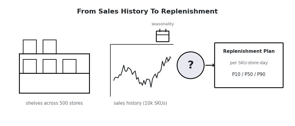
    Line-art scene: store shelves with products and a sales history curve flow into a question mark, producing a replenishment plan with P10, P50, and P90 quantities

    The Problem: thousands of SKUs across hundreds of stores. Predict each one’s future demand well enough to keep shelves full and waste low, then feed those numbers to replenishment and pricing.

    Answer

    The demand forecasting system ingests diverse data (sales, inventory, weather, promotions) and predicts product demand with ML models spanning time series, tree-based, and deep learning methods. It features a scalable layered architecture (data pipelines, real-time processing, integration for inventory management) and drives decisions with probabilistic forecasts, reducing stockouts, optimizing supply chains, and improving accuracy through iterative model training.

    (1) Problem Definition & Metrics: Fix granularity (SKU-store-day), horizon (2-week operational, 3-month tactical), and objective (minimize out-of-stocks and waste); measure with WMAPE and forecast bias.
    (2) Data Strategy: A unified feature store over internal signals (sales, hierarchy, pricing, promos, inventory, clicks) and external ones (calendar, weather, events, competitor, macro).
    (3) Layered Architecture: Ingestion → processing & feature store → modeling layer → serving APIs → monitoring & feedback.
    (4) Hierarchical Ensemble Modeling: Interpretable base (Prophet/ETS) at aggregate level, global LightGBM/XGBoost as the granular workhorse, TFT/DeepAR for high-volatility items, reconciled top-down and bottom-up.
    (5) Probabilistic Forecasts: Output quantile forecasts (P10, P50, P90) so logistics can set safety stock from uncertainty, not a single number.

    Five-layer architecture diagram: batch and real-time data ingestion flows to feature store, modeling layer, forecast serving API with replenishment and pricing consumers, and monitoring with a feedback arrow returning to modeling

    Figure 1: The five-layer system: ingestion and the feature store feed a model repository; forecasts are served through APIs to replenishment and pricing, while monitoring closes the loop back into retraining.

    Clarify Before Designing:
    (1) Scale: how many SKUs, stores, and series (SKU × store) must be forecast?
    (2) Granularity & Horizon: store-day or region-week? 2-week replenishment or 3-month tactical planning?
    (3) Decision Consumers: automated replenishment, or human planners reviewing suggestions?
    (4) Data Reality: is a promotions calendar available in advance? New product launch cadence (cold-start rate)?
    (5) Cost Asymmetry: the cost of a stockout (lost sale, empty shelf) versus overstock (waste, markdowns)?


    Login to view more content
  • MSD0006 Video Recommendation System


    How would you design a scalable and personalized video recommendation system for a platform like YouTube, Netflix, or TikTok that can recommend relevant videos in real time to billions of users?

    Line-art scene: a user with a phone facing a huge wall of video thumbnails labeled billions of videos, with a question mark leading to a clean top twenty feed on the phone

    The Problem: billions of videos, billions of users, one feed request at a time. Pick the top-20 most relevant videos for this user in milliseconds.

    Answer

    A modern recommendation system uses a multi-stage pipeline to narrow billions of videos down to a top-20 list for a user in milliseconds. It typically consists of Candidate Generation (filtering down to hundreds), Ranking (scoring those hundreds with deep learning), and Re-ranking (applying business logic for diversity, freshness, and safety). The full path is: Data Logging → Candidate Generation → Ranking → Re-ranking → Serving.

    (1) Multi-Stage Pipeline: No single model can score a billion items per request. The funnel makes it affordable: retrieve ~500 candidates cheaply, then rank precisely, then polish.
    (2) Data & Features: User signals (watch history, watch time, likes, skips, follows), video features (visual/audio/text embeddings, popularity, freshness), and context (time of day, device, network).
    (3) Candidate Generation: Multi-source retrieval (collaborative filtering / two-tower, content-based, seed-based co-watch, trending), merged and deduplicated to ~100-500.
    (4) Ranking: A deep model scores the candidates: DNNs on hundreds of features, Multi-Task Learning heads (click, watch time, like, share), and sequence models for session context.
    (5) Re-Ranking: Business and quality constraints: remove seen/unsafe items, inject diversity and freshness, fight filter bubbles.

    Funnel diagram: billions of videos narrow through candidate generation to about five hundred, through ranking to a top twenty list, then re-ranking and serving to the user feed

    Figure 1: The recommendation funnel: each stage trades breadth for precision: cheap retrieval cuts billions to hundreds, the ranking model orders them precisely, and re-ranking applies the final business logic before serving.

    Clarify Before Designing:
    (1) Scale: how many videos, daily active users, and feed requests per second?
    (2) Latency Budget: how many milliseconds for a feed request, end to end?
    (3) Objectives: what are we optimizing (clicks, watch time, long-term satisfaction), and are there multiple conflicting goals?
    (4) Cold Start Volume: how many new users and new videos arrive daily?
    (5) Constraints: ads insertion, content safety, regional/legal rules that override relevance?


    Login to view more content
  • MSD0005 Surveillance Video Anomaly Detection


    How would you design an end-to-end surveillance system that automatically detects and alerts security personnel to ‘anomalous events’ (e.g., break-ins, fainting, or prohibited movements) in a large shopping mall?

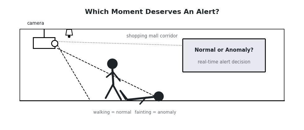
    Line-art scene: a shopping mall corridor watched by a wall-mounted camera, with a walking person and a question mark callout asking normal or anomaly

    The Problem: dozens of cameras stream continuously. Spot the rare anomalous event (break-in, fainting, prohibited movement) in real time, knowing you have no labeled anomalies to train on.

    Answer

    A surveillance anomaly detection system captures video streams, preprocesses them into clips, and uses a deep learning model (typically a pretrained video backbone plus a lightweight anomaly scoring head) to identify unusual behavior. It operates in a semi-supervised setup trained on normal data, runs in real time with sliding windows and temporal smoothing, and wraps the model in alerting, monitoring, and a human-in-the-loop feedback loop for calibration and retraining.

    (1) Ingestion & Preprocessing: Capture real-time streams from many cameras; resize frames and normalize pixels before clipping them into short windows.
    (2) Feature Extraction: A pretrained backbone (2D CNN (EfficientNet), optical flow, 3D CNN (I3D), or a Video Transformer (Swin, TimeSformer)) turns each clip into features.
    (3) Semi-Supervised Normal Model: An autoencoder or GAN trained on months of “normal” mall activity; high reconstruction error on new footage flags an anomaly against a calibrated threshold.
    (4) Alerting & Human-In-The-Loop: Real-time alerts send anomalous frames to operators, whose “Not an Anomaly” clicks feed recalibration and retraining.
    (5) System Design: Edge devices do preliminary processing to save bandwidth, the cloud does heavy computation; evaluation tracks precision, recall, F1 and false-alarm rates.

    Three-panel mechanism diagram: clips flow into a pretrained video backbone for feature extraction, an autoencoder trained on normal activity reconstructs them, and a reconstruction error curve crossing a threshold line flags anomalies

    Figure 1: The detection mechanism: backbone features feed a model trained to reconstruct normal activity; when reconstruction error crosses the calibrated threshold, the clip is flagged anomalous.

    Clarify Before Designing:
    (1) Scale: how many cameras, what fps and resolution, and how many concurrent clips must be scored?
    (2) Alert Latency: how many seconds from event to operator notification?
    (3) Anomaly Definition: a closed list of event types, or anything unusual; and are any labels available (frame-level, video-level, none)?
    (4) False-Alarm Budget: how many false alerts per camera per day can guards tolerate before they start ignoring the system?
    (5) Deployment: on-prem edge hardware available, or cloud-only?


    Login to view more content
  • DL0052 Rotary Positional Embedding

    What is Rotary Positional Embedding (RoPE)?

    Answer

    Rotary Positional Embedding (RoPE) encodes position by rotating each pair of query/key dimensions by an angle proportional to the token’s position, instead of adding a position vector. Because a rotation at position m composed with one at position n depends only on the difference, the attention dot product between tokens automatically reflects their relative distance, with no learned parameters and good length generalization. RoPE is the default in GPT-NeoX, LLaMA, PaLM, Qwen, and most modern LLMs.

    (1) Geometric Encoding: Each 2D slice of a query or key vector is rotated by m\theta_i, where m is the token position and \theta_i the per-dimension frequency.
    (2) Relative From Absolute: The dot product of two rotated vectors depends on (m - n)\theta_i only: absolute rotations yield relative-position attention.
    (3) Parameter-Free and Efficient: No embedding table, no attention bias, just a fixed trigonometric transform applied to Q and K.

    Mathematical Formulation:
    f(x, m) = \begin{pmatrix} \cos(m\theta) & -\sin(m\theta) \\ \sin(m\theta) & \cos(m\theta) \end{pmatrix} \begin{pmatrix} x_1 \\ x_2 \end{pmatrix}
    \theta_i = 10000^{-2i/d}

    Where:

    • m is the token’s absolute position in the sequence; x_1, x_2 are one 2D pair of the query/key vector.
    • \theta_i is the rotation frequency of the i-th dimension pair, geometrically decreasing across pairs so low dimensions capture short-range and high dimensions long-range offsets.
    Line chart of attention similarity versus relative token distance, with RoPE similarity decaying smoothly as distance grows while sinusoidal absolute positional encoding stays flat.

    Figure 1: Similarity vs relative distance: RoPE decays smoothly with distance (a built-in recency prior), while sinusoidal absolute PE stays roughly flat.

    Why It Won: RoPE is shift-invariant (the same rotation rule works at any position), adds zero parameters or memory, and, unlike learned absolute embeddings, degrades gracefully beyond the training length, which is why context-extension methods (NTK scaling, YaRN) all build on rescaling its frequencies.


    Login to view more content
  • DL0051 Sparsity in NN

    Explain the concept of “Sparsity” in neural networks.

    Answer

    Sparsity means that many of a network’s weights or activations are exactly zero. Sparse models are smaller to store, cheaper to run, and often more interpretable. It arises naturally (ReLU zeroes negative activations) or is induced deliberately through L1 regularization, pruning, or structured sparsity patterns designed for hardware acceleration.

    (1) Weight Sparsity: Pruning or L1 drives unimportant weights to zero, so the model keeps accuracy with a fraction of its parameters.
    (2) Activation Sparsity: ReLU produces zeros for all negative pre-activations, so only a subset of neurons “fire” per input.
    (3) Hardware Payoff: Only structured sparsity (e.g., NVIDIA’s 2:4 pattern: 2 zeros in every 4 values) maps to real speedups; scattered zeros alone rarely accelerate dense GPU kernels.

    Mathematical Formulation:
    \mathcal{L} = \mathcal{L}_{\text{task}} + \lambda \sum_i |w_i|
    \mathrm{ReLU}(x) = \max(0, x)

    Where:

    • w_i is the i-th model weight; the L1 penalty pushes small weights to exact zeros, with \lambda controlling sparsity strength.
    • x is a neuron’s pre-activation input; ReLU’s hard zero is the simplest source of activation sparsity.
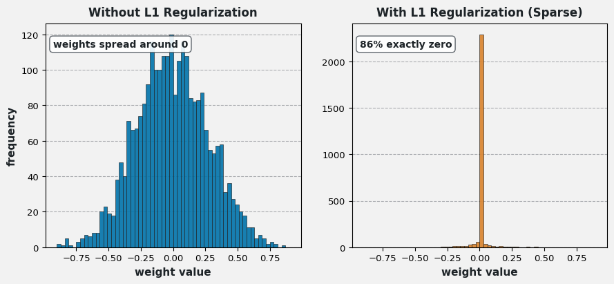
    Two weight-distribution histograms: without L1 a broad bell centered near zero, with L1 a tall spike at exact zero showing most weights pruned away.

    Figure 1: L1-induced weight sparsity: without L1 the weights form a broad bell; with L1 they collapse into a spike at exactly zero.

    Hardware Support (NVIDIA 2:4): Since Ampere (A100) and continuing in Hopper/Blackwell, Sparse Tensor Cores require every block of 4 values to contain at least 2 zeros (50% structured sparsity); they then skip the zero multiplies, doubling effective GEMM throughput and roughly halving the stored weights plus memory bandwidth.


    Login to view more content
  • MSD0004 Long Document Attention Scalability


    The standard Transformer’s self-attention mechanism has a computational and memory complexity of  O(N^2) , where  N is the sequence length. For long document classification (e.g., thousands of tokens), this quadratic scaling becomes prohibitive.

    Describe one or more attention modifications you would design or choose to enable efficient and effective long document classification.

    Problem framing diagram: a full N by N attention matrix labeled O of N squared memory flows into a question mark, with the target sub-quadratic attention at equal classification accuracy

    The Problem: full self-attention costs O(N^2) in compute and memory. Redesign attention so a several-thousand-token document stays affordable without giving up classification accuracy.

    Answer

    To handle long documents, the quadratic complexity of full self-attention (O(N^2)) must be reduced. The two primary directions are Sparse Attention (Longformer, BigBird), which constrains each token to a relevant subset (a local window plus a few global tokens), and Hierarchical Attention (HATN), which applies attention within segments first and then across segment representations. Both preserve classification quality while cutting cost from O(N^2) toward linear; linearized and recurrent variants (Performer, Linformer, Transformer-XL) attack the same wall from other angles.

    (1) Sparse Attention (Mechanism): Replace the full attention matrix with a sparse design: local window attention for nearby context plus global tokens (e.g., [CLS]) that exchange information with all tokens (Longformer, BigBird).
    (2) Hierarchical Attention (Structure): Split the document into segments; apply token-level attention within each segment, then a document-level attention across segment representations (HATN, LNLF-BERT).
    (3) Linearized / Recurrent Variants: Kernel approximations (Performer, Linformer) reach true linear complexity; Transformer-XL / Compressive Transformer carry a recurrent memory across segments.

    Two attention matrices side by side in grayscale: full attention with every cell filled, and sliding window attention with only a diagonal band of width five filled

    Figure 1: Full attention (left) fills the whole N \times N matrix; sliding-window attention (right) keeps only a diagonal band: each token attends to its neighbors, and cost drops from O(N^2) to O(N \cdot w).

    Clarify Before Designing:
    (1) Document Length: typical and maximum token count: 2k, 8k, 32k?
    (2) Starting Point: adapt a pretrained BERT-style encoder, or train from scratch?
    (3) Binding Constraint: memory at training, or latency at inference?
    (4) Interaction Pattern: does classification need global token interactions (a [CLS] readout), and how long-range are the dependencies?
    (5) Budget For Change: may we modify the architecture, or only fine-tune an off-the-shelf long model?


    Login to view more content
  • MSD0003 Spam Email Detection


    Design an end-to-end Machine Learning system to effectively detect and filter spam emails in a high-volume email service.

    Describe how you would design, train, and deploy this system.

    Line-art scene: a stream of email envelopes flows into a filter marked with a question mark, splitting into a clean inbox and a spam bin

    The Problem: a high-volume mail stream must be split into inbox and spam in real time, where one false positive can lose a user’s important email forever.

    Answer

    The system is a real-time classification pipeline at the mail gateway. It begins with data collection and preprocessing (features from text and metadata) and trains a supervised model on user-labeled history. Deployment is a low-latency prediction service that scores every incoming email and applies a tuned threshold. Because spammers constantly adapt, the system lives or dies by its monitoring and continuous-training loop that fights concept drift.

    (1) Objectives & Metrics: Precision first: a false positive (legitimate mail in spam) is far costlier than a false negative; keep recall high as the secondary goal and track F1 / PR-AUC.
    (2) Data & Features: User-labeled history plus external corpora; features span email text (subject, body), metadata (sender, domain reputation, recipients), and behavior (links, attachments, frequency).
    (3) Two-Stage Cascade: A fast traditional model filters the obvious ~80%, then a Transformer deep-analyzes the ambiguous ~20%: accuracy where it matters, speed everywhere else.
    (4) Deployment: A low-latency prediction API at the gateway: receive → extract features → score → threshold → route to spam folder or inbox.
    (5) Maintenance: Monitor precision/recall daily, harvest user feedback (‘Mark as Spam’ / ‘Not Spam’) as fresh labels, and retrain continuously against concept drift.

    Inference pipeline: incoming email passes through mail server, spam API, feature extraction, model scoring, then a threshold decision branching to spam folder or inbox

    Figure 1: The real-time inference path: every incoming email is scored by the model (e.g., 0.95), and a tuned threshold (e.g., 0.8) routes it (spam folder or inbox) inside the latency budget of the mail gateway.

    Clarify Before Designing:
    (1) Scale: email volume per day and peak QPS at the gateway?
    (2) Latency Budget: how many milliseconds may scoring add before the email is delivered?
    (3) Cost Asymmetry: confirmed: is a false positive (lost legitimate mail) really the catastrophic error here?
    (4) Labels: how much user-labeled spam/not-spam data exists, and how fresh is it?
    (5) Adversaries: how quickly do spam tactics mutate in this ecosystem: days, weeks?


    Login to view more content
  • MSD0002 Image to Video Classification


    You are given a pretrained image classification network, such as ResNet. How would you adapt it to perform video classification, ensuring that both spatial and temporal information are captured?

    Please discuss possible architectural modifications and trade-offs between different approaches.

    Problem framing diagram: a pretrained 2D ResNet that sees frames independently flows into a question mark, with the target video classification requiring both spatial and temporal cues

    The Problem: a pretrained 2D CNN understands each frame in isolation. Fill the question mark with an adaptation that adds temporal modeling without throwing away what the image network already knows.

    Answer

    The missing ingredient is temporal modeling: a 2D CNN sees each frame independently, so any adaptation must add a mechanism that aggregates information across time. Three families cover the design space: inflate the network into 3D convolutions, keep the 2D CNN as a per-frame encoder and add a sequence model on top, or simply pool or attend over per-frame features. The right choice trades temporal modeling power against compute cost and data hunger.

    (1) 3D CNNs (C3D / I3D): Extend 2D convolutions into 3D to learn motion directly; I3D inflates pretrained 2D filters into 3D, keeping ImageNet weights useful.
    (2) CNN + Sequence Model: Use the 2D CNN as a per-frame feature extractor, then run an LSTM / TCN / Transformer over the feature sequence for temporal modeling.
    (3) Temporal Pooling / Attention: Aggregate per-frame features with average/max pooling or attention: cheapest, but frame order and fine motion cues fade.

    Mechanism diagram of the CNN plus sequence model option: four video frames each pass through the same pretrained CNN, producing a stack of feature vectors that flows into an LSTM or Transformer temporal model, producing the class prediction

    Figure 1: The CNN + sequence model option: the pretrained 2D CNN is reused per frame, and a temporal model (LSTM/TCN/Transformer) learns how features evolve. This is the balanced default: full ImageNet leverage, moderate cost, natural variable-length handling.

    Clarify Before Designing:
    (1) Latency: real-time or offline? What is the per-clip inference budget?
    (2) Input Statistics: fps, clip duration, resolution: trimmed clips or untrimmed streams?
    (3) Data Scale: how much labeled video is available: hundreds or hundreds of thousands of clips?
    (4) Compute: can training and inference afford 3D-convolution cost?
    (5) Motion Sensitivity: do classes depend on subtle motion (opening vs closing) or mostly on scenes and objects?


    Login to view more content