What are dilated convolutions? When would you use them?
Answer
Dilated convolutions enhance standard convolution by inserting gaps between filter elements, thereby allowing the network to gather more context (a larger receptive field) without an increase in parameters or a reduction in resolution.
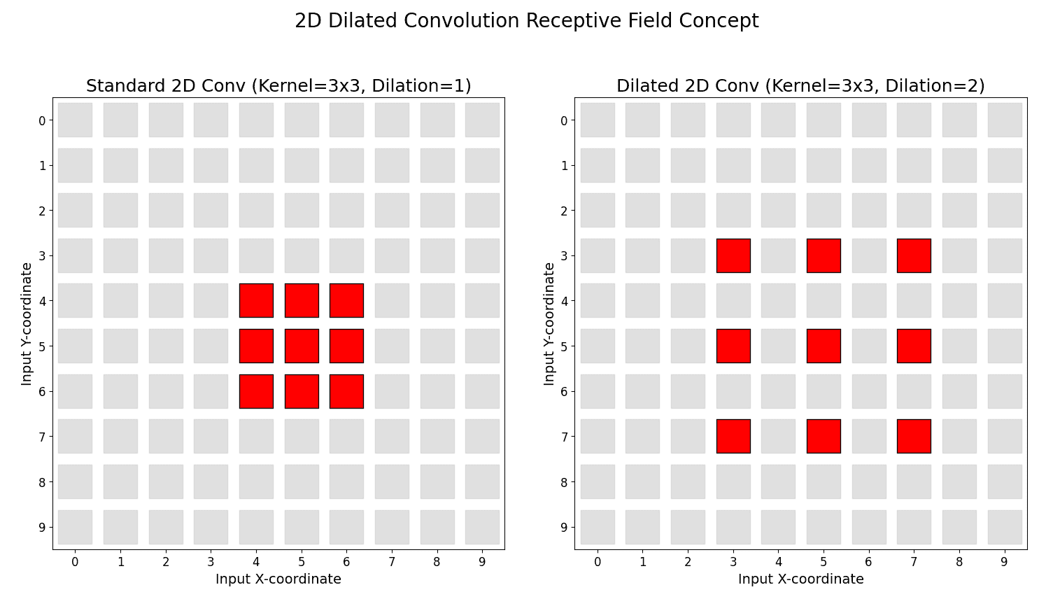
Dilated convolutions (also known as atrous convolutions) modify standard convolution by inserting gaps (zeros) between kernel elements. A “dilation rate” dictates the spacing of these gaps. A dilation rate of 1 is a standard convolution.
Contrast with Pooling:
Pooling reduces spatial resolution (downsamples) while increasing the receptive field.
Dilated convolutions increase the receptive field without reducing resolution.
Multi-Scale Feature Extraction:
By adjusting the dilation rate, these convolutions can aggregate features from both local neighborhoods and larger regions, making it easier for the network to learn from multi-scale context.
Common Use Cases: Any task needing large receptive fields without downsampling.
(1) Semantic segmentation (e.g., DeepLab): Expand the receptive field and capture multi-scale context.
(2) Audio processing (e.g., WaveNet): Model long-range temporal dependencies.
Here is a 1D Dilated Convolution illustration.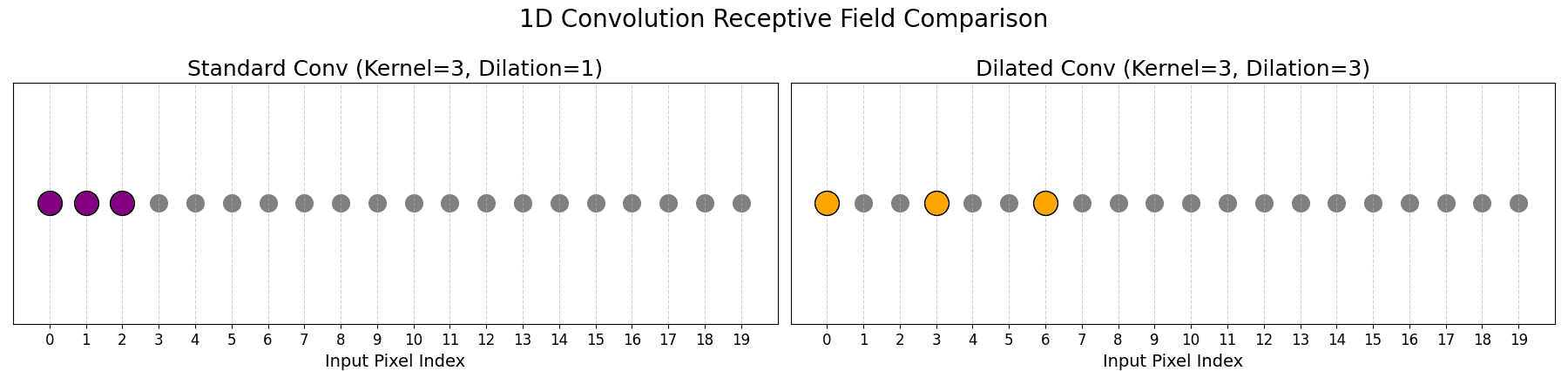
Here is a 2D Dilated Convolution illustration.