Please explain the concept of “Attention Mechanism.”
Answer
The attention mechanism is a technique in neural networks that allows the model to focus on specific parts of the input sequence when making predictions. It addresses the limitation of traditional sequence-to-sequence models that compress an entire input sequence into a single fixed-size context vector, which can lose information, especially for long sequences.
Attention lets the model dynamically decide which parts of the input are most important for each output step. For each output token, attention computes a weighted sum over all input tokens. These weights represent how much “attention” the model should pay to each input.
Key Components:
Query (Q): Represents what we are looking for or the current element being processed.
Key (K): Represents what information is available from the input.
Value (V): The actual information content to be extracted if a key matches the query.
Each output uses a query to compare with keys and then uses the scores to weight values.
Calculation (Scaled Dot-Product Attention):
Similarity Score: Calculated by taking the dot product of the Query with each Key.
Scaling: The scores are scaled down by the square root of the dimension of the keys ( ) to reduce variance and prevent large values from pushing the Softmax function into regions with tiny gradients.
Normalization: Normalized into a probability distribution using the Softmax function. Ensures the weights sum to 1.
Weighted Sum: Multiplied by the Values to get the final attention output.

Where: : Matrices of queries, keys, and values.: Dimension of key vectors.
 : Converts similarity scores to probabilities.
The plot below shows how much “attention” each input token receives in a simplified attention mechanism. It uses softmax-normalized weights over a 5-token sentence.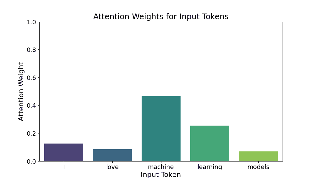
 ) using rules of thumb (default heuristics), then tune via cross-validation or out-of-bag (OOB) error to find the best value for your specific dataset.

 = total number of features,
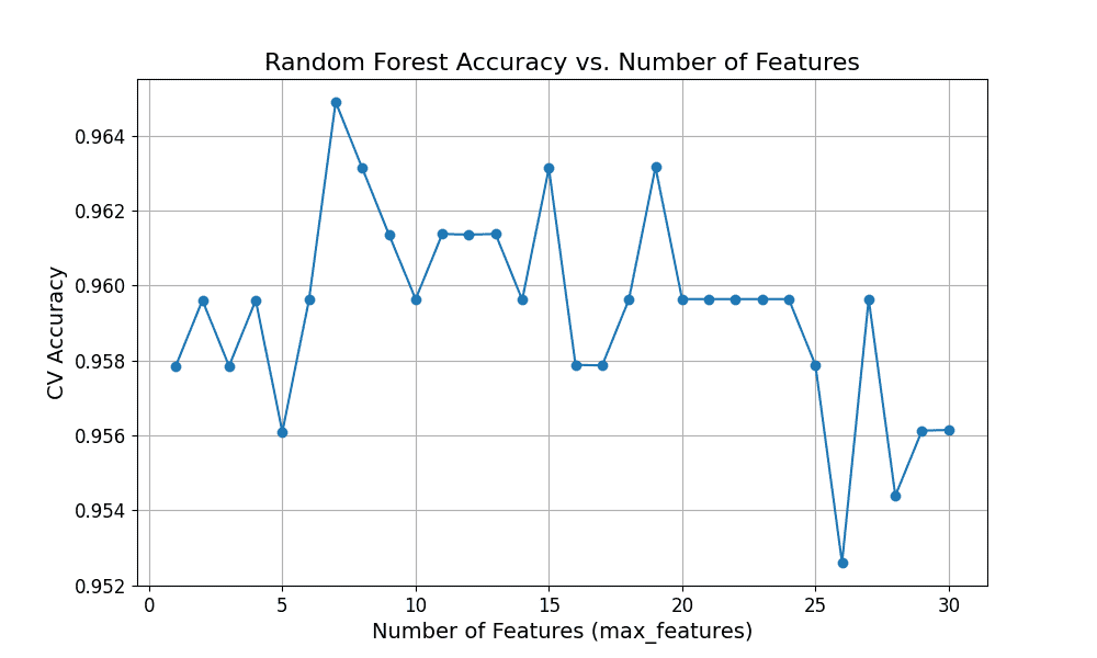

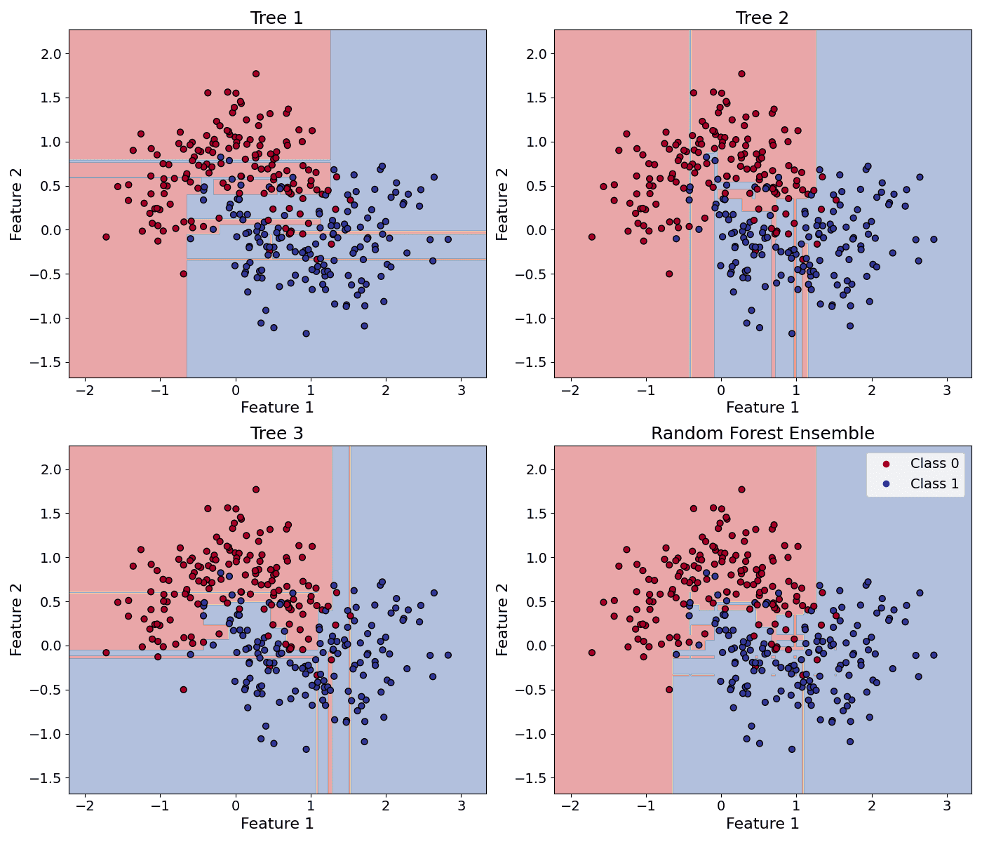
 = prediction of the b-th tree.
 = total number of trees.

 nearest neighbors. The majority votes for classification. Average of values for regression.
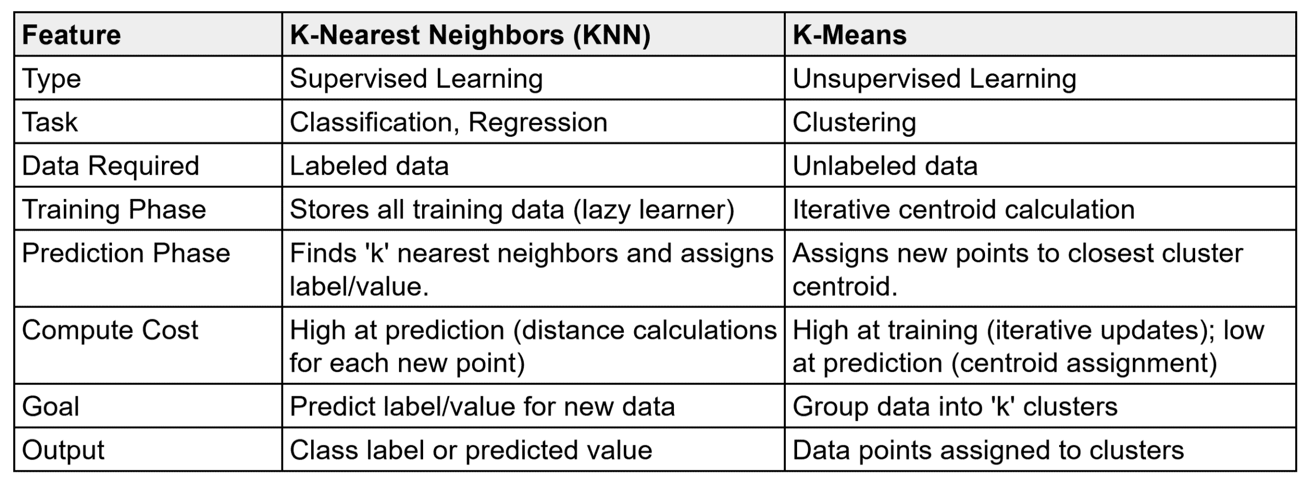

 is cluster
  ,
,  is its centroid.
 can be calculated by the following equation.
 = intra-cluster distance,
 = nearest-cluster distance.
 is the set of points in cluster
  is the centroid of cluster
  is a data point assigned to cluster
 uniformly at random from the dataset.
 , compute its squared distance to the nearest chosen centroid:
 is one of the already chosen centroids.
 with probability:
 is the squared distance from point
  is the sum of minimum squared distances from all data points to their nearest chosen centroid.

 is the data point.
 is the cluster center.
