Category: Medium

DL0091 Quantization Formats

What is quantization (FP16/BF16/INT8/INT4), and how does it affect model memory and accuracy?

Answer

Quantization stores weights, activations, or KV-cache entries in a numeric format with fewer bits than the FP32 values the model was defined in, trading numerical resolution for memory and bandwidth. Memory falls almost exactly linearly in bit width: a 70B-parameter model occupies 280 GB in FP32, 140 GB in FP16 or BF16, 70 GB in INT8, and roughly 37 GB in 4-bit with group scales. The two 16-bit floating formats differ only in how they split the 16 bits: FP16 spends 5 bits on the exponent and 10 on the mantissa (max magnitude 65,504, so gradients can overflow without loss scaling), while BF16 keeps FP32’s 8 exponent bits and truncates the mantissa to 7, giving the full $10^{38}$ dynamic range at coarser resolution. Below 16 bits the formats become integers plus a scale, so a real number is recovered as $\hat{w} = s(w_q - z)$ , and quality now depends on how finely those scales are estimated. In practice INT8 weights are essentially free in accuracy with per-channel scales, INT4 weight-only costs a few tenths of a perplexity point on a 70B model with a good calibration method, and quantizing activations is the hard part because transformer activations contain a handful of channels with magnitudes 20x to 100x the median.

(1) Exponent Versus Mantissa: FP16 and BF16 use the same 16 bits, but BF16’s 8 exponent bits buy dynamic range at the cost of precision, which is why BF16 is the default training format on modern accelerators and needs no loss scaling.
(2) Memory Is Linear In Bits: parameter memory is $N b / 8$ bytes, so each halving of the bit width halves the checkpoint, the resident weights, and the bytes moved per token.
(3) Integers Need A Scale And A Granularity: per-tensor scaling is cheapest, per-channel is the practical minimum for weights, and group-wise (typically 128 weights per scale) is what makes 4 bits usable.
(4) Weight-Only Helps Because Decode Is Bandwidth-Bound: single-stream generation reads every weight per token, so 4-bit weights cut latency even when the matmul itself runs in FP16 after dequantization.
(5) Error Concentrates In Outliers: a single extreme value stretches the scale and destroys resolution for every other value in the group, which is why outlier handling matters more than the nominal bit count.

Bit-field diagram comparing FP32, FP16, BF16, FP8 E4M3, INT8 and INT4: each format is drawn as a proportional bar split into sign, exponent and mantissa fields, with dynamic-range notes on the right

Figure 1: Bit budgets drawn to scale. BF16 keeps FP32’s 8 exponent bits and pays with 7 mantissa bits, FP16 does the reverse, and the sub-8-bit formats drop the exponent entirely in favour of an external scale factor.

An integer format is defined by an affine map from the real line onto $2^b$ evenly spaced levels. Symmetric quantization fixes the zero-point at $z = 0$ and is the standard choice for weights, whose distribution is roughly zero-centred; asymmetric quantization keeps a learned $z$ and suits post-ReLU or post-GELU activations that sit mostly on one side of zero. The granularity of $s$ is the real design knob: one scale per tensor stores nothing extra but is destroyed by a single outlier channel, whereas one scale per group of $g = 128$ weights adds a 16-bit scale and a 16-bit zero-point per group, which raises an INT4 tensor from 4.0 to 4.25 effective bits. Calibration methods such as GPTQ and AWQ then choose the rounding of each weight to minimise the error of the layer output on a small calibration set rather than the error of the weight itself, which is what closes most of the remaining gap at 4 bits.

Mathematical Formulation:
$\hat{w} = s (w_q - z)$
$w_q = \mathrm{clip}(\mathrm{round}(w/s) + z,\ 0,\ 2^b - 1)$
$s = \frac{\max(w) - \min(w)}{2^b - 1}$
$b_{eff} = b + \frac{32}{g}$
$M = \frac{N \, b_{eff}}{8}$

Where:

$\hat{w}$ is the dequantized value actually used in the matmul, and $w$ is the original FP32 or BF16 weight.
$w_q$ is the stored integer code, clipped into $\{0,\ldots,2^b-1\}$ ; values outside the calibrated range are saturated rather than wrapped.
$s$ is the scale (step size) and $z$ the zero-point; symmetric quantization sets $z = 0$ and uses $s = \max|w| / (2^{b-1} - 1)$ .
$b$ is the nominal bit width and $g$ the group size, the number of weights sharing one $(s, z)$ pair stored in FP16, hence the $32/g$ overhead.
$b_{eff}$ is the effective bits per weight; with $b = 4$ and $g = 128$ this gives $b_{eff} = 4.25$ .
$N$ is the parameter count and $M$ the weight memory in bytes; for $N = 7 \times 10^{10}$ this is about 37 GB. Required condition: $s > 0$ must be computed from calibration data before any activation quantization is applied.

Bar chart of weight memory in gigabytes for a 70 billion parameter model: 280 GB in FP32, 140 GB in FP16 or BF16, 70 GB in INT8 and 37 GB in INT4 with group size 128, with a dashed line marking the 80 GB capacity of one GPU

Figure 2: Weight memory for a 70B model. Only the 4-bit variant fits one 80 GB GPU with room left for the KV cache, and because decoding is memory-bandwidth bound the same reduction shows up directly in tokens per second.

Property	FP16	BF16	INT8	INT4 (g=128)
Layout	1 sign, 5 exponent, 10 mantissa	1 sign, 8 exponent, 7 mantissa	8-bit integer plus a per-channel FP16 scale	4-bit integer plus a scale per 128 weights
Dynamic range	Max 65,504; underflows below 6e-5	Same as FP32, about 3.4e38	256 levels inside the calibrated range	16 levels per group; clipping is the main risk
70B weights	140 GB	140 GB	70 GB	About 37 GB at 4.25 effective bits
Typical role	Inference, and training with loss scaling	Default training and master-weight format	W8A8 serving at high batch, compute-bound prefill	Weight-only decode on capacity-limited GPUs
Accuracy cost	None measurable for inference	None measurable; the lost mantissa bits rarely matter	Under 1% with per-channel scales and outlier handling	A few tenths of perplexity on 70B, clearly worse below 7B
Hardware support	Tensor cores on every recent GPU	Ampere onward, plus TPUs	Roughly 2x the FP16 matmul throughput	No native 4-bit matmul on most GPUs; kernels dequantize in registers

August 16, 2026

DL0090 Post-Training vs Quantization-Aware Training

What is the difference between post-training quantization and quantization-aware training, and how would you choose between them when shipping a model to an on-device NPU?

Answer

Post-training quantization (PTQ) takes a finished float checkpoint and converts it to low precision after the fact: a few hundred unlabeled samples are pushed through the network so the tool can observe activation ranges, pick a scale and zero point per tensor or per channel, and round the weights. No labels, no loss, no backward pass, and typically minutes to a couple of hours on a single GPU. Quantization-aware training (QAT) instead inserts fake-quantization nodes into the graph and continues training, so every forward pass sees rounded values while gradients flow through the non-differentiable rounding step via the straight-through estimator (STE). The one-line distinction worth memorizing: PTQ fits the quantizer to fixed weights, while QAT moves the weights to fit the quantizer. At INT8 on a well-behaved network the two land within a few tenths of a point of each other, so PTQ wins on cost; at 4 bits and below, or on outlier-heavy and depthwise-separable models, PTQ falls off a cliff and QAT recovers most of the loss.

(1) Where It Happens: PTQ is a post-processing step on a frozen checkpoint; QAT is a fine-tuning stage that must run inside your training pipeline with the original data loader and loss.
(2) What Data It Needs: PTQ needs only a small calibration set (roughly 128 to 1024 unlabeled samples) that is representative of deployment traffic; QAT needs labeled data, or at least a teacher model for distillation.
(3) The STE Trick: rounding has zero gradient almost everywhere, so QAT pretends the quantizer is the identity inside the clipping range and passes the gradient straight through, which is what lets weights drift toward values that round well.
(4) Where PTQ Breaks: per-tensor scales collapse when channel ranges differ by orders of magnitude (depthwise convolutions), when activations carry massive outliers (transformer residual streams), or when the bit width drops to 4 or fewer.
(5) Decision Rule: always try PTQ first because it is cheap and reversible; escalate to QAT only when a measured accuracy gap survives per-channel scales, better range selection, and bias correction.

Mechanically, a fake-quant node applies quantize → dequantize in the forward pass, so tensors stay in float during QAT but carry exactly the values the integer kernel will produce at inference. That means QAT does not speed up training; it slows it down by 20 to 40 percent while simulating the deployment numerics. The payoff is that the optimizer sees the rounding error as part of the loss surface and settles into flatter minima where a few least significant bits do not matter. PTQ has no such feedback: whatever error the rounding introduces is simply propagated forward, which is why its failure mode is a sudden collapse rather than a graceful slide.

Two horizontal pipelines. Top row, post-training quantization: trained FP32 checkpoint, calibration pass on 128 to 1024 unlabeled samples, fit scale and zero point, export INT model. Bottom row, quantization-aware training: trained FP32 checkpoint, insert fake-quant nodes, fine-tune with labels and STE gradients, fold scales and export INT model.

Figure 1: The same checkpoint, two routes to integer inference. PTQ adds one forward-only calibration pass; QAT adds a full fine-tuning loop whose gradients reach the weights through the straight-through estimator.

Mathematical Formulation:
$s = \frac{x_{max} - x_{min}}{2^{b} - 1}$
$q = \mathrm{clip}(\lfloor x/s \rceil + z, 0, 2^{b} - 1)$
$\hat{x} = s\,(q - z)$
$\frac{\partial \mathcal{L}}{\partial x} \approx \frac{\partial \mathcal{L}}{\partial \hat{x}} \cdot \mathbf{1}[x_{min} \leq x \leq x_{max}]$

Where:

$\hat{x}$ is the dequantized value the network actually computes with, and $x$ is the original float weight or activation.
$s$ is the scale and $z$ the zero point (the integer that maps to exactly 0.0); $q$ is the stored integer code.
$b$ is the bit width, so $b = 8$ gives 256 levels and $b = 4$ only 16; $x_{min}, x_{max}$ are the calibrated clipping bounds, chosen per channel for weights and per tensor or per token for activations.
$\lfloor \cdot \rceil$ is round-to-nearest and $\mathrm{clip}$ saturates values outside the representable range; both are the source of the error being managed.
The last line is the straight-through estimator: the indicator $\mathbf{1}[\cdot]$ passes the gradient unchanged inside the clipping range and zeroes it outside, which is the only reason QAT can backpropagate through rounding.
PTQ solves for $s, z$ with $x$ held fixed; QAT keeps the whole chain in the graph and updates $x$ (and, with learned-step methods, $s$ itself).

Line chart of top-1 accuracy versus bit width from INT8 down to INT2. PTQ tracks the FP32 baseline at INT8 and INT6 but drops to 68 at INT4, 41 at INT3 and 6 at INT2, while QAT stays at 74.5 at INT4, 71 at INT3 and 62 at INT2.

Figure 2: Illustrative accuracy versus bit width. The two methods are indistinguishable at INT8, which is why PTQ dominates production INT8 pipelines; the gap opens abruptly at 4 bits and below, where the rounding error stops behaving like small additive noise.

Dimension	Post-Training Quantization	Quantization-Aware Training
Data needed	128 to 1024 unlabeled calibration samples	Labeled training data or a teacher for distillation
Compute	Minutes to hours, one GPU, forward passes only	Hours to days, often multi-GPU, full training loop
Pipeline access	Works on a vendor or third-party checkpoint	Requires the original recipe, loss and hyperparameters
Typical INT8 result	Within roughly 0.5 points of FP32 with per-channel weights	Essentially lossless, rarely worth the cost
Typical INT4 result	Large drop unless advanced methods (GPTQ, AWQ) are used	Recovers most of the gap, the standard choice below 4 bits
Iteration speed	Cheap to sweep many bit widths and granularities	Each configuration is a separate training run

August 15, 2026

DL0088 PEFT: Parameter-Efficient Fine-Tuning

Compare Parameter-Efficient Fine-Tuning (PEFT) methods: LoRA, adapters, and prompt/prefix tuning. When would you choose each?

Answer

All three families freeze the pretrained weights and train a tiny set of new parameters, but they differ in where those parameters live, and that single structural choice decides inference cost, serving flexibility, and achievable quality. LoRA adds a low-rank update in parallel to existing weight matrices, so after training the update folds back into $W$ and costs exactly zero extra latency. Serial adapters insert a small bottleneck MLP inside the block’s forward path, which keeps task modules cleanly composable but adds depth, so every decoded token pays for them. Prefix and prompt tuning touch no weight matrix at all: prefix tuning prepends trainable key/value vectors at every layer, prompt tuning prepends trainable vectors only at the input embeddings, which is the cheapest option in parameter count but the least stable and it consumes context length. In practice LoRA is the default (paired with 4-bit quantization as QLoRA when GPU memory is the binding constraint), adapters win when modular composition matters more than latency, and prefix/prompt tuning wins when the base weights must stay byte-identical or when you want per-request conditioning.

(1) Where The Parameters Live: LoRA sits parallel to chosen projections, adapters sit serially between sublayers, prefix tuning sits in the KV cache rather than in any weight tensor.
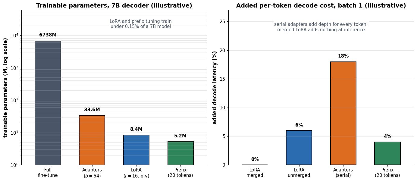
(2) Mergeability Decides Latency: only LoRA is exactly mergeable into $W_0$ ; adapters add two matmuls and a nonlinearity per sublayer that cannot be folded away, which is a 10-25% decode overhead at batch 1 on a 7B model.
(3) Capacity Is A Knob, Except For Prompts: rank $r$ and bottleneck width $b$ scale capacity smoothly, while prompt tuning’s capacity saturates and only becomes competitive with full fine-tuning above roughly 10B parameters.
(4) Multi-Tenant Serving: unmerged LoRA and prefix tuning both support heterogeneous batching (per-request low-rank gather, or per-request KV prefix) from one frozen base copy; merged LoRA needs a separate weight copy per task and adapters need a weight swap per request.

Diagram of one transformer block: input, LayerNorm, self-attention, LayerNorm, FFN, output. A blue LoRA box below attention taps the same input and adds its output back in parallel, a green prefix-tuning box above attention prepends trainable key and value vectors, and an orange serial adapter box sits in the path between the FFN and the block output

Figure 1: The three injection sites in one block. LoRA is parallel and therefore mergeable, the adapter is serial and therefore always in the critical path (real adapter recipes place one after attention and one after the FFN), and prefix tuning changes only K and V, leaving every weight untouched.

Two consequences are worth stating precisely because interviewers probe them. First, the merge is algebraically exact, not an approximation: $W_0 + (\alpha/r)BA$ is just another matrix of the same shape, so a merged LoRA checkpoint is indistinguishable from a normally fine-tuned one at serving time, and the price is that you can no longer swap tasks without unmerging. Second, PEFT saves optimizer and gradient memory, not activation memory: with Adam you drop from roughly 12-16 bytes per trainable parameter of state to almost none, which is why a 7B model fine-tunes on a single 24GB card, but activations still scale with batch size and sequence length, and QLoRA’s 4-bit NF4 base plus paged optimizers is what pushes a 65B model onto one 48GB GPU. Prefix tuning has a third quirk: because the prefix occupies KV slots, a 20-token prefix at every layer permanently shortens the usable context and its quality is non-monotonic in prefix length, which is why the original work needed a reparameterization MLP to train stably at all.

Mathematical Formulation:
$h = W_0 x + \frac{\alpha}{r} B A x$
$W' = W_0 + \frac{\alpha}{r} B A$
$h = x + W_{\mathrm{up}} \sigma(W_{\mathrm{down}} x)$
$\tilde{K} = \mathrm{concat}(P_k, K)$
$\tilde{V} = \mathrm{concat}(P_v, V)$

Where:

$h$ is the sublayer output and $x$ the input; $W_0$ is the frozen pretrained matrix of shape $d_{out} \times d_{in}$ .
$B \in \mathbb{R}^{d_{out} \times r}$ and $A \in \mathbb{R}^{r \times d_{in}}$ are the LoRA factors with rank $r \ll \min(d_{in}, d_{out})$ ; $A$ is Gaussian-initialized and $B$ is zero-initialized so training starts from the pretrained function.
$\alpha$ is a scaling constant, and the ratio $\alpha/r$ keeps the effective update magnitude roughly stable when you sweep $r$ ; $W'$ is the merged weight used at inference.
$W_{\mathrm{down}} \in \mathbb{R}^{b \times d}$ and $W_{\mathrm{up}} \in \mathbb{R}^{d \times b}$ form the adapter bottleneck of width $b$ , with nonlinearity $\sigma$ ; the residual term $x$ plus near-zero initialization makes the adapter an approximate identity at step 0.
$P_k, P_v \in \mathbb{R}^{p \times d_k}$ are the per-layer, per-head prefix key and value vectors of length $p$ ; $K, V$ are the ordinary projected keys and values, so attention runs over $p + n$ positions for a sequence of length $n$ .

Two-panel bar chart. Left panel, log scale: trainable parameters for full fine-tuning 6738M, adapters 33.6M, LoRA 8.4M, prefix tuning 5.2M. Right panel: added per-token decode latency at batch 1, merged LoRA 0 percent, unmerged LoRA 6 percent, serial adapters 18 percent, prefix tuning 4 percent

Figure 2: Illustrative budgets for a 7B decoder with $d = 4096$ and 32 layers. Parameter counts span three orders of magnitude, yet the latency picture is unrelated to them: the smallest method is not the fastest, and merged LoRA is free.

Dimension	LoRA	Serial Adapters	Prefix / Prompt Tuning
Insertion point	Parallel to chosen linear layers (q,v by default; all attention and FFN projections for hard tasks)	Serial bottleneck after the attention and FFN sublayers	Extra K/V vectors at every layer (prompt tuning: input embeddings only)
Trainable share (7B)	0.05-0.5% (8.4M at r=16 on q,v)	0.5-3% (33.6M at b=64, two per layer)	Under 0.1% (5.2M for a 20-token prefix)
Mergeable	Yes, algebraically exact	No, extra depth is irreducible	No, but no weight is modified either
Inference cost	0% merged; roughly 5-10% unmerged at batch 1	Roughly 10-25% at batch 1, worst at small batch	Small KV cost, but the prefix permanently shortens usable context
Many tasks, one base	Strong: keep unmerged and batch a per-request low-rank gather	Weak: needs a per-request module swap, though AdapterFusion composes trained modules	Strong: a prefix is just cached K/V, trivially per-request
Quality on hard tasks	Matches full fine-tuning closely at adequate rank; underfits at very low r on large domain shifts	Comparable to LoRA, with a well-studied bottleneck-width knob	Lags on generation and reasoning; unstable below roughly 10B parameters
Choose it when	Default choice; memory-bound runs pair it with 4-bit QLoRA; hundreds of task variants over one base	You want modular, composable, independently versioned task modules and have latency headroom	Base weights must stay immutable, or you need cheap per-request conditioning at very large scale

August 15, 2026

DL0086 LoRA: Low-Rank Adaptation

What is LoRA, and can you explain the low-rank decomposition idea and why it is parameter-efficient?

Answer

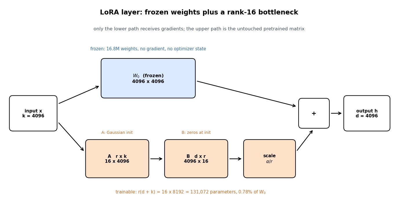
LoRA (Low-Rank Adaptation) freezes every pretrained weight matrix and learns only a rank-constrained update beside it: instead of training $W_0 + \Delta W$ with a full $d \times k$ update, it factors the update as $\Delta W = BA$ with $B \in \mathbb{R}^{d \times r}$ , $A \in \mathbb{R}^{r \times k}$ and $r \ll \min(d,k)$ . The motivation is the intrinsic-dimension hypothesis: adapting a large pretrained model to a downstream task moves the weights along a very low-dimensional subspace, so a rank-8 or rank-16 correction captures almost all of the useful change. For one $4096 \times 4096$ attention projection, a rank-16 factorization trains 131,072 numbers instead of 16.8M, roughly 0.78% of the matrix. The efficiency that matters in practice is not forward FLOPs, which barely change, but optimizer and gradient state: Adam keeps two moments plus an fp32 master copy per trainable parameter, so shrinking the trainable set by two or three orders of magnitude is what turns a multi-node job into a single-GPU job. At inference the product can be folded back with $W' = W_0 + (\alpha/r)BA$ , so a merged LoRA adds zero latency compared with the original model.

(1) Frozen Base, Additive Branch: the pretrained matrix never receives a gradient; all learning happens in the parallel $BA$ branch whose output is added to the frozen path.
(2) Rank Is The Budget Knob: parameter count is $r(d+k)$ and grows linearly in $r$ , while the full matrix costs $dk$ , so the ratio is tiny for any practical rank.
(3) Zero Initialization On One Factor: $A$ gets a random Gaussian init and $B$ is initialized to zeros, so $\Delta W = 0$ at step 0 and training starts exactly at the pretrained function.
(4) Memory Savings Come From Optimizer State: gradients and Adam moments exist only for adapter parameters, which is where the 8x reduction in peak training memory comes from, not from cheaper matrix multiplies.
(5) Mergeable And Swappable: a task adapter is a few tens of MB, so many tasks can share one frozen base, either merged per deployment or batched as separate adapters in a single server.

Diagram of a LoRA layer: the input feeds a frozen 4096 by 4096 projection on the upper path and a rank-16 bottleneck A then B then alpha over r scaling on the lower path, with both paths summed into the output

Figure 1: A LoRA layer keeps the frozen 16.8M-parameter projection untouched and routes the input through a rank-16 bottleneck whose 131,072 trainable parameters are added back, scaled by $\alpha/r$ .

Two implementation details do most of the work. The scaling factor $\alpha/r$ decouples the effective update magnitude from the rank, so raising $r$ to add capacity does not silently multiply the learning rate on the adapter branch; the common convention is to fix $\alpha$ and sweep $r$ . The choice of target modules matters more than the rank in most experiments: the original paper adapted only the attention query and value projections, while current practice applies LoRA to all linear layers including the MLP, which raises trainable parameters to about 42M on an 8B model but consistently closes the gap to full fine-tuning. One caveat on merging: if the base weights are quantized, folding a bf16 adapter into a 4-bit matrix reintroduces quantization error, so quantized deployments usually keep the adapter separate.

Mathematical Formulation:
$h = W_0 x + \Delta W x$
$\Delta W = \frac{\alpha}{r} B A$
$|\Theta| = r(d + k)$
$\rho = \frac{r(d + k)}{d k}$
$W' = W_0 + \frac{\alpha}{r} B A$

Where:

$h$ is the layer output and $x \in \mathbb{R}^{k}$ the input activation for one token.
$W_0 \in \mathbb{R}^{d \times k}$ is the frozen pretrained matrix, and $\Delta W$ is the learned correction.
$B \in \mathbb{R}^{d \times r}$ and $A \in \mathbb{R}^{r \times k}$ are the trainable factors; the rank $r$ satisfies $r \ll \min(d,k)$ , which forces $\mathrm{rank}(\Delta W) \leq r$ .
$\alpha$ is a fixed scaling constant, so $\alpha/r$ keeps the update magnitude roughly rank-independent.
$|\Theta|$ is the trainable count per adapted matrix and $\rho$ its fraction of the full matrix; with $d = k = 4096$ and $r = 16$ this gives 131,072 parameters and $\rho \approx 0.0078$ .
Required initial condition: $B = 0$ with $A$ Gaussian, so $\Delta W = 0$ before the first step; the last line is the merge applied after training.

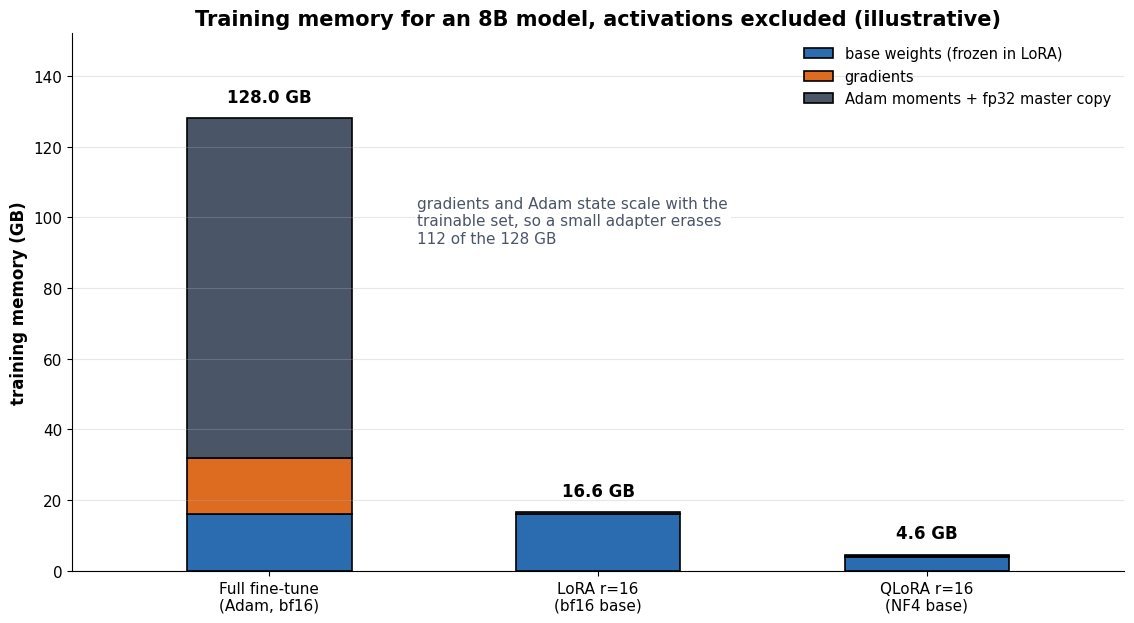
Stacked bar chart of training memory in gigabytes for an 8B model: full fine-tuning totals 128 GB from 16 GB base weights, 16 GB gradients and 96 GB optimizer state, LoRA rank 16 totals 16.6 GB, and QLoRA with a 4-bit base totals 4.6 GB

Figure 2: Illustrative training memory for an 8B model before activations: full fine-tuning spends 96 GB on Adam state alone, LoRA with 41.9M trainable parameters needs about 16.6 GB, and a 4-bit frozen base drops that to about 4.6 GB.

Property	LoRA	Full Fine-Tuning	Bottleneck Adapters
Trainable parameters (8B model)	41.9M at r=16 on all linear layers, about 0.5%	8.0B, all of them	Comparable order, set by bottleneck width
Added inference latency	None once merged into the base weights	None	Extra sequential layers, noticeable at small batch
Peak training memory	About 17 GB, or 5 GB with a 4-bit base	About 128 GB with Adam in mixed precision	Similar to LoRA
Multi-task serving	Hundreds of small adapters over one frozen base, batchable	One 16 GB checkpoint per task	Swappable but cannot be merged away
Quality ceiling	Matches full tuning on most instruction and style adaptation	Upper bound, clearly better for large domain shift	Roughly on par, less used today

August 15, 2026

DL0084 RAG: Retrieval-Augmented Generation

What is RAG (retrieval-augmented generation), and describe the components of a RAG pipeline?

Answer

Retrieval-augmented generation conditions a frozen language model on text fetched at query time from an external corpus, so the answer is grounded in documents the model never memorized. Nothing about the weights changes: the retriever supplies evidence, the prompt carries it, and the decoder writes an answer that should be traceable to that evidence. This buys three things a fine-tuned model cannot easily give you, namely freshness (reindex a document and the next query sees it), attribution (each claim can cite a chunk ID), and access control (metadata filters keep a user out of documents they may not read). A practical pipeline has an offline half and an online half: the offline half runs chunk → embed → index, and the online half runs retrieve → rerank → assemble prompt → generate. The parts that decide whether the system works in production are rarely the LLM; they are the chunking policy, the hybrid retrieval that combines dense and lexical matching, and the cross-encoder reranker that decides which five of fifty candidates actually reach the context window.

(1) Ingestion and Chunking: parse the source into text, then split it into passages of roughly 400 to 800 tokens with modest overlap, attaching metadata (document ID, section, timestamp, ACL tags) that later powers filtering and citation.
(2) Embedding and Indexing: a bi-encoder maps each chunk to a fixed vector stored in an ANN index (HNSW or IVF-PQ) alongside a sparse BM25 or SPLADE index, because dense and lexical retrieval fail on different queries.
(3) Query Processing and Retrieval: the query is optionally rewritten (decontextualized against chat history, expanded, or decomposed for multi-hop), encoded once, and used to pull a wide candidate set of 30 to 100 chunks from both indexes, fused by reciprocal rank fusion.
(4) Reranking and Context Assembly: a cross-encoder scores each query-chunk pair jointly and keeps the top 3 to 8, which are deduplicated, ordered, and packed into the prompt with instructions to answer only from the provided context and to cite chunk IDs.
(5) Generation, Evaluation, and Guardrails: the LLM generates a grounded answer, and an offline harness tracks retrieval recall@k separately from answer faithfulness, since a wrong answer with perfect retrieval and a right answer with broken retrieval demand opposite fixes.

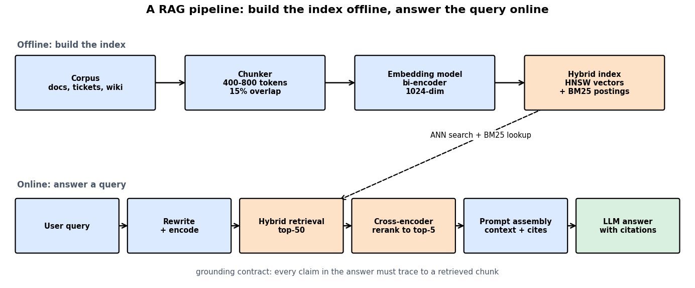
Two-row diagram: the offline row runs corpus to chunker to embedding model to a hybrid index of HNSW vectors plus BM25 postings; the online row runs user query to rewrite and encode to hybrid retrieval of top-50 candidates to a cross-encoder rerank to top-5 to prompt assembly to LLM answer with citations, with a dashed arrow from the index down to the retrieval stage

Figure 1: The offline half builds a hybrid index once per document revision; the online half spends its latency budget on retrieval, reranking, and decoding, and only the reranked top-5 chunks ever enter the context window.

Most RAG failures are retrieval failures, so it helps to measure each stage separately. A useful decomposition is recall@50 for the first-stage retriever (did the answer-bearing chunk survive at all?) and recall@5 after reranking (did it reach the prompt?). Dense bi-encoders miss exact identifiers such as error codes, part numbers, and rare acronyms, which BM25 handles trivially; BM25 misses paraphrases, which the bi-encoder handles. Fusing the two lists and then letting a cross-encoder read query and chunk together typically removes a large share of the remaining misses, at the cost of one extra model call over 50 pairs, which is why the reranker runs on the shortlist and never on the corpus.

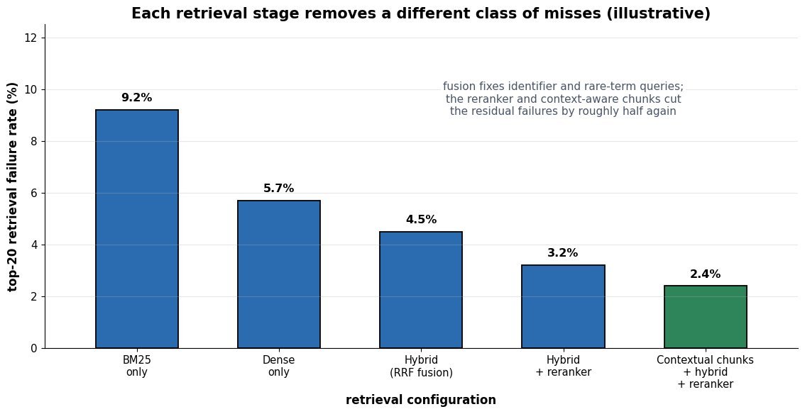
Bar chart of top-20 retrieval failure rate for five configurations: BM25 only at 9.2 percent, dense only at 5.7 percent, hybrid fusion at 4.5 percent, hybrid plus reranker at 3.2 percent, and contextual chunk embeddings plus hybrid plus reranker at 2.4 percent

Figure 2: Illustrative stage-by-stage gains: hybrid fusion fixes the queries dense retrieval alone drops, and the cross-encoder reranker plus context-aware chunk embeddings cut the residual failure rate further.

Mathematical Formulation:
$s(q,c) = \frac{e_q^{\top} e_c}{\|e_q\|\,\|e_c\|}$
$\mathcal{R}_k(q) = \text{top-}k\{\, s(q,c) : c \in \mathcal{D} \,\}$
$\mathrm{RRF}(c) = \sum_{r=1}^{R} \frac{1}{K + \mathrm{rank}_r(c)}$
$p(y \mid q) = \prod_{t=1}^{T} p_\theta(y_t \mid y_{1:t-1}, q, \mathcal{R}_k(q))$

Where:

$s(q,c)$ is the cosine similarity between the query embedding $e_q$ and the chunk embedding $e_c$ , both produced by the same bi-encoder.
$\mathcal{D} = \{c_1,\ldots,c_M\}$ is the chunked corpus with $M$ passages, and $\mathcal{R}_k(q)$ is the retrieved set of size $k$ that the prompt will carry.
$\mathrm{RRF}(c)$ fuses $R$ ranked lists (dense, lexical, and any filtered variants); $\mathrm{rank}_r(c)$ is the position of chunk $c$ in list $r$ , and the constant $K \approx 60$ damps the influence of top ranks so one confident list cannot dominate.
$p_\theta$ is the frozen decoder, $y_t$ the token at step $t$ of a $T$ -token answer; the retrieved set enters only as prompt context, so $\theta$ is never updated by indexing new documents.
In practice the ANN index returns an approximate $\mathcal{R}_k$ : HNSW recall is tuned by the search-width parameter, and quantized indexes trade a small recall loss for roughly $4\times$ to $8\times$ less memory.

Dimension	RAG	Fine-tuning	Long-Context Stuffing
Best for	Large, changing, permissioned corpora	Style, format, task behavior, domain jargon	Small corpora that fit in one window
Update cost	Reindex the changed chunks, seconds	A new training run per refresh	None, but every request pays for the tokens
Attribution	Native: cite the retrieved chunk ID	None, facts are diffused into weights	Possible, but no ranking signal to audit
Main failure mode	Retriever misses the answer-bearing chunk	Confident stale answers, catastrophic forgetting	Lost-in-the-middle, cost and latency growth
Serving complexity	High: index, retriever, reranker, eval harness	Low at serve time, high at train time	Low, especially with prompt caching

August 15, 2026

DL0081 Tokenizer Vocabulary Size Effects

How does the tokenizer vocabulary size affect LLM model quality, memory, and throughput?

Answer

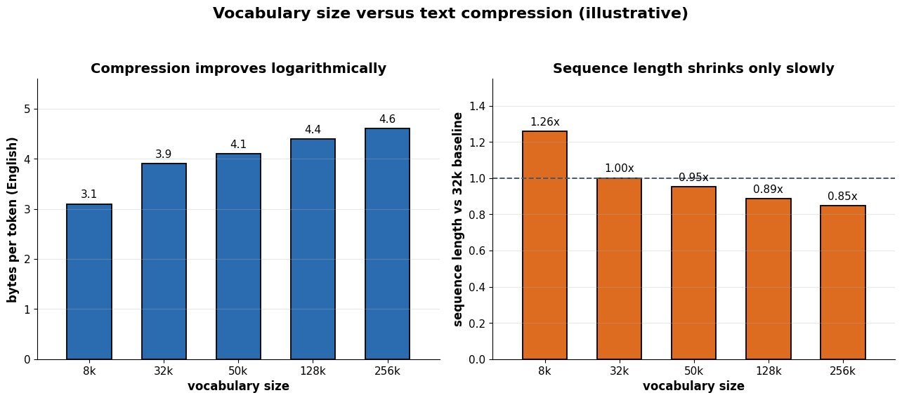
Vocabulary size $V$ is one of the few hyperparameters that moves quality, memory, and throughput in opposite directions at the same time, so there is a genuine optimum rather than a “bigger is better” rule. On the cost side, the embedding and unembedding tables grow linearly in $V$ (up to $2Vd$ parameters when untied), the output projection adds $2Vd$ FLOPs per token, and the training-time logits tensor of shape $b \times T \times V$ in fp32 becomes one of the largest activations in the whole model. On the benefit side, a larger vocabulary compresses text into fewer tokens, which shortens sequences, shrinks the KV cache, cuts the $O(T^2)$ attention term, and reduces the number of autoregressive decode steps needed to emit the same text. The catch is that compression improves only logarithmically in $V$ while cost grows linearly, and each added token gets a smaller slice of the training signal, so rare embeddings end up undertrained. Empirically the optimum grows with model size: 32k was reasonable for GPT-2-era models, Meta’s Llama 3 moved to 128,256 tokens, and Google’s Gemma 2 uses 256,128, while byte-level and byte-patch models sit at the opposite extreme.

(1) Memory Cost Is Linear: at $d = 4096$ and $V = 128\text{k}$ , untied tables hold about 1.05B parameters, roughly 13% of an 8B model, and 2.1 GB of bf16 weights before optimizer state.
(2) Compression Gain Is Logarithmic: going 32k → 128k buys only about 11% fewer tokens per document in English, while the embedding tables quadruple.
(3) The Output Softmax Dominates Small Models: the $d \times V$ projection is about 7% of forward FLOPs for an 8B model but roughly a third for a 1B model with $d = 2048$ .
(4) Quality Is Non-Monotonic: too small and sequences are long and multilingual fertility explodes; too large and rare rows receive too few gradient updates, producing dead or glitch tokens.
(5) Throughput Has Two Units: tokens per second falls slightly as $V$ grows, but bytes (or words) per second usually rises because fewer steps are needed for the same text.

Two bar panels: left panel shows bytes per token rising from 3.1 at 8k vocabulary to 3.9 at 32k, 4.1 at 50k, 4.4 at 128k and 4.6 at 256k; right panel shows relative sequence length for a fixed document falling from 1.26 at 8k to 1.00 at 32k, 0.95 at 50k, 0.89 at 128k and 0.85 at 256k

Figure 1: Illustrative English compression: quadrupling the vocabulary from 32k to 128k lifts bytes per token from 3.9 to 4.4, which shortens sequences by only about 11%, while the embedding tables grow 4x.

The most under-appreciated cost is not the weights but the logits activation. Cross-entropy is normally computed in fp32, so a single 8192-token sequence against a 128k vocabulary materializes $8192 \times 128000 \times 4$ bytes, about 4.2 GB, and a microbatch of four pushes past 16 GB before the backward pass. This is why large-vocabulary training runs adopt chunked or fused cross-entropy kernels that never hold the full logits matrix, and why teams sometimes cap $V$ purely for activation-memory reasons. At inference the picture flips: the vocabulary contributes a fixed $d \times V$ GEMM per decode step, which is cheap relative to the KV-cache reads in a large model, and the shorter sequence means fewer steps overall, so end-to-end latency for generating a fixed passage typically improves. A separate trap is evaluation: validation loss is not comparable across tokenizers, because the per-token loss is defined over a different unit of text, so comparisons must be normalized to bits per byte or bits per character.

Mathematical Formulation:
$P_{emb} = 2 V d$
$T = B / c(V)$
$c(V) \approx a + \beta \log V$
$C = 6 (N_{nv} + P_{emb}) T$
$M_{logits} = b \, T \, V \, p$
$V^{\star} \propto N_{nv}^{0.83}$

Where:

$P_{emb}$ is the parameter count of the input embedding plus output unembedding; the factor 2 drops to 1 when the two are tied.
$V$ is the vocabulary size and $d$ the model width; $N_{nv}$ is the non-vocabulary (attention plus MLP) parameter count.
$B$ is the raw text size in bytes, $c(V)$ the compression ratio in bytes per token, and $T$ the resulting token count; $a$ and $\beta$ are corpus- and language-dependent fit constants.
$C$ is approximate training FLOPs under the $6ND$ rule, which is why a larger $V$ both adds parameters and removes tokens.
$M_{logits}$ is the logits activation in bytes, with microbatch $b$ and precision $p$ (4 for fp32); $V^{\star}$ is the compute-optimal vocabulary, whose exponent near 0.83 means it grows more slowly than the rest of the model.

Two U-shaped curves of relative loss in bits per byte versus vocabulary size on a log-2 axis from 4k to 256k: the 300M non-embedding parameter curve bottoms out near 24k, and the 7B curve sits lower overall and bottoms out near 96k, showing the optimum shifting right with model size

Figure 2: Illustrative shape of the trade-off at fixed compute: loss measured in bits per byte is U-shaped in $V$ , and the minimum shifts right as non-embedding capacity grows, because a bigger body can afford to spend parameters on the vocabulary.

Property	Small BPE (32k)	Large BPE (128k-256k)	Byte level (256)
Bytes per token (English)	about 3.9	about 4.4 to 4.6	1.0
Embedding params at d=2048, untied	131M	525M to 1.05B	1M
fp32 logits per 8192-token sequence	1.05 GB	4.2 GB to 8.4 GB	8 MB
Average updates per row over 300B tokens	about 9M	about 1M to 2M	over 1B
Sequence length for a fixed document	baseline	0.85x to 0.89x	about 3.9x
Main weakness	High fertility on non-English text and code	Undertrained rare rows, huge logits activation	Long sequences, many decode steps
Best fit	Sub-1B on-device models, single-language domains	Multilingual frontier models with long contexts	Noisy input, character tasks, patch-based research

August 15, 2026

DL0080 Tokenization in LLMs

Explain tokenization in large language models.

Answer

Tokenization is the reversible mapping between raw text and the sequence of integer ids a language model actually consumes, drawn from a fixed vocabulary of size $V$ . Modern LLMs use subword vocabularies that sit between characters (short vocab, very long sequences) and words (huge vocab, unavoidable out-of-vocabulary gaps), and the dominant recipe is byte-level BPE: count adjacent symbol pairs over a training corpus, greedily merge the most frequent pair, and repeat until the vocabulary reaches its target size. Because the base alphabet is the 256 possible bytes rather than Unicode characters, any input is representable and there is no UNK token, at the cost of spending several tokens per character on scripts the merge table never learned. The tokenizer is frozen before pretraining and is effectively part of the architecture: it fixes the embedding matrix and output projection ( $2Vd$ parameters), it decides how many model passes a sentence costs, and it determines whether the model sees 1024 as one symbol or three. Most surprising LLM behaviors around arithmetic, non-English cost, and trailing whitespace trace back to this layer rather than to the transformer itself.

(1) Subword Is A Middle Ground: character-level models keep the vocabulary tiny but inflate sequence length, and attention is $O(N^2)$ in that length; word-level vocabularies need hundreds of thousands of entries and still miss rare words and typos.
(2) How BPE Is Trained And Applied: training produces an ordered merge list; encoding replays those merges greedily on each pretokenized chunk, so segmentation is deterministic and not a search over the best split.
(3) Pretokenization Comes First: in the GPT-style recipe a regex splits text on whitespace, punctuation, and digit groups before BPE runs, which is why the leading space belongs to the token (" the" and "the" are different ids) and why, with standard pretokenization, merges do not cross word boundaries; that constraint comes from the pretokenizer rather than from BPE itself, and implementations that skip or relax it (see SuperBPE below) do learn multi-word tokens.
(4) Vocabulary Size Is A Compute Knob: raising $V$ lowers fertility (tokens per word) so each sentence needs fewer forward passes, but it grows the embedding and softmax cost, which is why the field drifted from 32k to 128k vocabularies (Llama 2 → Llama 3) as models got larger.
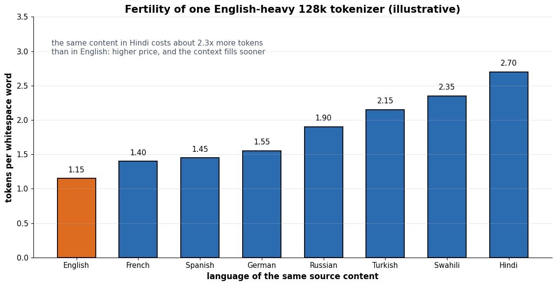
(5) The Failure Modes Users Notice: digit grouping degrading arithmetic, non-English prompts costing two to three times more tokens for the same content, glitch tokens whose embeddings were barely trained, and special chat-template ids that must never be injectable from user text.

Bar chart of tokens per whitespace word for eight languages under one English-heavy tokenizer: English 1.15, French 1.40, Spanish 1.45, German 1.55, Russian 1.90, Turkish 2.15, Swahili 2.35, Hindi 2.70

Figure 1: Illustrative fertility gap: with a merge table dominated by English text, the same content in Hindi consumes roughly $2.3\times$ more tokens, so it costs more per request and reaches the context limit sooner.

Two implementation details matter more in production than the choice of merge algorithm. First, digit handling: tokenizers that merge arbitrary digit runs give the model inconsistent units for numbers, so 2024, 202, and 24 share no stable structure and column-wise arithmetic has to be learned per token; Llama 3 and several recent tokenizers instead force digits into groups of at most three, and some research tokenizers split every digit. Second, special tokens such as beginning-of-text and end-of-turn markers are inserted out of band by the chat template, not produced by BPE over user text; if a serving layer lets a user string encode into those ids, the model’s turn structure can be rewritten from inside a prompt. Related traps include unnormalized Unicode (NFC versus NFKC changes ids for accented text), tokenizer and checkpoint version skew, which silently shifts every embedding lookup, and untrained vocabulary rows that surface as glitch tokens the model cannot repeat back.

Mathematical Formulation:
$(a,b)^{*} = \arg\max_{(a,b)} c(a,b)$
$F = \frac{T}{W}$
$P_{\text{emb}} = 2 V d$
$C_{\text{word}} = F \cdot (C_{\text{body}} + 2 V d)$

Where:

$(a,b)^{*}$ is the pair chosen at each BPE training step, and $c(a,b)$ is its frequency as adjacent symbols in the corpus; the merge is appended to an ordered list that encoding later replays.
$F$ is fertility: $T$ tokens produced for $W$ whitespace words, measured per language and per corpus, so it is a property of the tokenizer and the text, not of the model.
$P_{\text{emb}}$ counts the input embedding plus the untied output projection for vocabulary $V$ and hidden width $d$ ; tying the two halves this term but couples input and output geometry.
$C_{\text{word}}$ is the compute per word of text, where $C_{\text{body}}$ is the per-token cost of everything except the vocabulary layers; the two $V$ -dependent effects pull in opposite directions, which is why an interior optimum in $V$ exists and grows with model size.

Two panels versus vocabulary size on a log axis: left panel shows tokens per word falling from about 1.72 at 4k vocab to 1.27 at 512k with diminishing returns, right panel shows relative compute per word dipping to a minimum near 33k vocabulary and rising to about 1.65 at 512k

Figure 2: Illustrative trade-off for a 1B-scale model with $d = 1024$ : shorter sequences from a larger vocabulary stop paying for themselves once the $2Vd$ output-layer cost rivals the transformer body, and the minimum shifts right as $d$ and depth grow.

Feature	Byte-level BPE	WordPiece	Unigram LM
How the vocab is learned	Greedily merge the most frequent adjacent pair, recording an ordered merge list	Merge the pair that most increases corpus likelihood under a unigram model	Start from a large candidate set and prune the tokens whose removal costs the least likelihood (EM)
How text is segmented	Replay merges in training order; deterministic and fast	Longest-match-first greedy scan, with `##` marking continuations	Viterbi search for the most probable segmentation, and it can sample splits for subword regularization
Unseen input	No UNK is possible; the 256-byte alphabet covers all of Unicode	Emits UNK for characters outside the alphabet unless byte fallback is added	Byte fallback is optional in SentencePiece and usually enabled
Where you see it	GPT-2 onward, Llama, Mistral, Qwen	BERT and the encoder family that followed it	T5, ALBERT, and many multilingual encoders

August 15, 2026

DL0078 LLM Training Stages

What are the standard stages of LLM training?

Answer

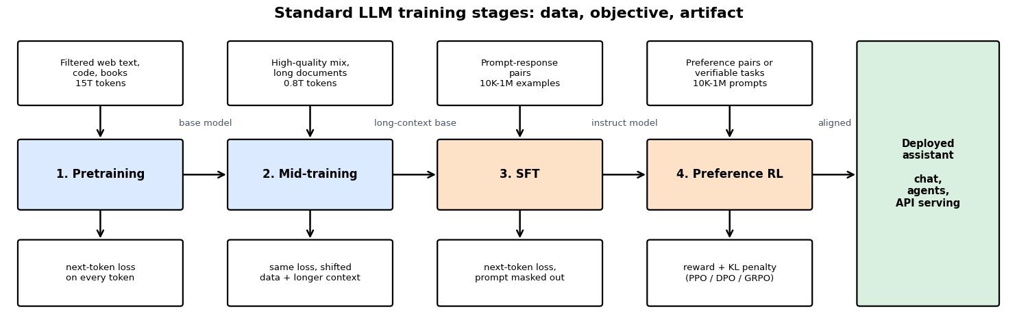
A modern LLM is built in a sequence of stages that share one architecture but differ in data, objective, and scale: pretraining on a web-scale corpus with next-token prediction, an increasingly explicit mid-training phase that reweights the data mix and extends the context window, supervised fine-tuning (SFT) on curated prompt-response pairs, and preference optimization that turns human or programmatic judgments into a training signal (reward model plus PPO, DPO, or reinforcement learning with verifiable rewards). The split is not cosmetic: pretraining consumes well over 90% of the total tokens and FLOPs and is where almost all knowledge and reasoning capacity is acquired, while post-training uses a tiny fraction of the compute to select and expose behaviors the base model already has. Each stage produces a named artifact that the next stage consumes, so the usual lineage is base model → long-context base → instruct model → aligned model. Practical pipelines also interleave evaluation, safety filtering, distillation, and quantization, but those are packaging steps rather than new learning objectives.

(1) Pretraining: self-supervised next-token loss on trillions of filtered web, code, and book tokens, run once at enormous cost; this stage fixes the tokenizer, the parameter count, and the knowledge cutoff.
(2) Mid-Training: continued pretraining on a higher-quality mix with upsampled math, code, and long documents, plus context-length extension and learning-rate annealing, using roughly 1-10% of the pretraining tokens.
(3) Supervised Fine-Tuning: the same cross-entropy loss but computed only on response tokens with the prompt masked out, teaching format, instruction following, and tool-call syntax from $10^4$ to $10^6$ curated examples.
(4) Preference Optimization: optimizes a reward (learned from pairwise comparisons, or computed by a verifier) under a KL penalty toward the SFT reference policy, which is what shifts a model from plausible to preferred.
(5) Compute Asymmetry: post-training is cheap, so it is where iteration happens; anything that requires new knowledge or a longer context has to go back to a pretraining-style stage.

Four-stage LLM training pipeline: filtered web text feeds pretraining with a next-token loss producing a base model, a high-quality long-document mix feeds mid-training producing a long-context base, prompt-response pairs feed SFT with the prompt masked producing an instruct model, and preference pairs or verifiable tasks feed preference RL with a reward plus KL penalty, yielding a deployed assistant

Figure 1: The four canonical stages with their input data, objective, and output artifact. Only the data distribution and loss mask change between stages 1 to 3; stage 4 replaces likelihood with a reward under a KL constraint.

Mathematical Formulation:
$\mathcal{L}_{\mathrm{PT}}(\theta) = -\sum_{t=1}^{T} \log p_{\theta}(x_t \mid x_{1:t-1})$
$\mathcal{L}_{\mathrm{SFT}}(\theta) = -\sum_{t \in \mathcal{A}} \log p_{\theta}(y_t \mid x, y_{1:t-1})$
$\mathcal{L}_{\mathrm{RM}}(\phi) = -\log \sigma\big(r_{\phi}(x,y_w) - r_{\phi}(x,y_l)\big)$
$J(\theta) = \mathbb{E}\big[r_{\phi}(x,y)\big] - \beta\,\mathrm{KL}(\pi_{\theta}\,\|\,\pi_{\mathrm{ref}})$

Where:

$x_{1:t-1}$ is the preceding context and $x_t$ the target token, so pretraining averages this loss over every position of every document.
$x$ is the prompt, $y$ the response, and $\mathcal{A}$ the set of assistant token positions; positions outside $\mathcal{A}$ are masked, which is the only structural difference between SFT and pretraining.
$y_w$ and $y_l$ are the preferred and rejected responses for the same prompt, $r_{\phi}$ is the reward model, and $\sigma$ is the logistic function, giving the Bradley-Terry pairwise objective.
$\pi_{\theta}$ is the policy being trained and $\pi_{\mathrm{ref}}$ the frozen SFT checkpoint; the KL term is what keeps generations fluent instead of collapsing onto reward-model artifacts.
$\beta > 0$ sets the strength of that anchor: small $\beta$ permits reward hacking, large $\beta$ leaves the model barely changed from SFT.

Log-scale bar chart of training tokens per stage: pretraining 15 trillion tokens at 94.9 percent, mid-training 0.8 trillion at 5.1 percent, SFT 0.2 billion at 0.001 percent, and preference RL 4 billion at 0.03 percent

Figure 2: Illustrative token budget for a frontier-scale run. Pretraining and mid-training together see about 99.97% of all tokens, so post-training cannot add missing knowledge, only elicit and shape what is already in the weights.

Post-Training Option	Reward Model + PPO	DPO	Verifiable Rewards (GRPO)
Signal required	Pairwise human preferences, then a learned scalar reward	Pairwise preferences used directly, no reward model	A programmatic checker: unit tests, math answer match, schema validity
Models held in memory	Four: policy, reference, reward, critic	Two: policy and frozen reference	Two plus a sampler: no critic, group baseline replaces it
Online generation	Yes, rollouts dominate wall-clock time	No, offline on a fixed pair dataset	Yes, several samples per prompt
Main failure mode	Reward hacking and length inflation once the reward model is over-optimized	Off-policy drift: pairs stop reflecting the current policy, likelihood of both responses can fall	Only works where correctness is checkable; gaming the checker instead of the task
Typical use	Broad helpfulness and safety at frontier labs with annotation pipelines	Small teams, quick style and tone alignment on limited GPUs	Math, code, and reasoning models where long chains of thought pay off

August 15, 2026

DL0077 LLM Prediction Objective

What is a large language model, and what is its prediction objective?

Answer

A large language model (LLM) is a neural network, in practice a decoder-only Transformer with billions of parameters, trained on trillions of tokens of text to model the probability distribution over token sequences. Its prediction objective is next-token prediction: factor the sequence probability with the chain rule and maximize the log-likelihood of each observed token given its left context, which is identical to minimizing cross-entropy over the vocabulary at every position. The training signal is self-supervised, since the label at position $t$ is simply the token at position $t+1$ , so no human annotation is required and one sequence of length $T$ yields $T-1$ supervised examples in a single forward pass, or a full $T$ when a leading BOS token supplies the context for the first real token. Everything an LLM appears to know (syntax, factual associations, translation, arithmetic, code structure) is a byproduct of driving that one loss down, because accurately predicting the next token over a broad corpus requires modeling the processes that generated the text. Base pretraining optimizes likelihood only; instruction following and refusal behavior come later, from supervised fine-tuning and preference optimization, which change the objective rather than the architecture.

(1) What Makes It “Large”: parameter count in the billions, a training corpus in the trillions of tokens, and a compute budget allocated according to scaling laws, so capability improvements are largely predictable from loss curves rather than architectural novelty.
(2) The Objective Is Autoregressive: the chain-rule factorization plus a causal mask means position $t$ may only attend to positions $1$ through $t$ , which is what makes single-pass training and left-to-right generation consistent with each other.
(3) Loss Is Cross-Entropy Over the Vocabulary: the final layer projects the hidden state to $V$ logits, softmax turns them into a distribution, and the loss is the negative log-probability of the single correct token.
(4) Perplexity Is the Reported Metric: $\mathrm{PPL} = \exp(\mathcal{L})$ is the effective branching factor, so a mean loss of $2.3$ nats means the model is about as uncertain as choosing uniformly among 10 tokens; perplexity depends on the tokenizer and is not comparable across different vocabularies.
(5) Likelihood Is Not Helpfulness: maximizing the likelihood of scraped text also rewards reproducing its errors and its style, and teacher forcing never trains the model to recover from its own mistakes, which is the origin of exposure bias.

Bar chart of a next-token distribution after the prefix The capital of France is: Paris receives 0.83, the receives 0.04, a receives 0.021, now 0.015, located 0.012, and the remaining roughly 50000 tokens share 0.082

Figure 1: Illustrative output of one position: a full distribution over the whole vocabulary. Because the observed continuation is “Paris” with probability 0.83, this position contributes $-\ln 0.83 \approx 0.19$ nats to the loss.

Two properties of this objective explain most of how LLMs are trained and evaluated. First, supervision is dense: the causal mask lets one forward pass score every shifted position simultaneously, so a 2048-token document produces 2047 gradient contributions (2048 with a BOS prepended), which is why raw web text is enough to train a model with hundreds of billions of parameters. Second, the loss is a strictly proper scoring rule on the token distribution, so the gradient pushes probability mass toward the observed token and away from every competitor at once; the model is never told which wrong token was “almost right”. That makes the loss an excellent optimization target and a poor proxy for downstream quality, which is why teams track perplexity for training health but use task benchmarks and human preference for release decisions.

Mathematical Formulation:
$p_{\theta}(x_1,\ldots,x_T) = \prod_{t=1}^{T} p_{\theta}(x_t \mid x_{1:t-1})$
$p_{\theta}(\cdot \mid x_{1:t-1}) = \mathrm{softmax}(W h_t + b)$
$\mathcal{L}(\theta) = -\frac{1}{T}\sum_{t=1}^{T} \log p_{\theta}(x_t \mid x_{1:t-1})$
$\mathrm{PPL} = \exp\big(\mathcal{L}(\theta)\big)$

Where:

$x_1,\ldots,x_T$ is the token sequence produced by the tokenizer, and $x_{1:t-1}$ is the left context of position $t$ ; the first line is the chain-rule factorization that defines an autoregressive model.
The $t=1$ term assumes a leading BOS token as context; without it the empty-context term is dropped and the sum runs over $T-1$ positions with the mean taken over $T-1$ terms.
$h_t \in \mathbb{R}^{d}$ is the final-layer hidden state at position $t$ , and $W \in \mathbb{R}^{V \times d}$ with bias $b$ is the unembedding head, frequently weight-tied to the input embedding.
$V$ is the vocabulary size (roughly 128k for Llama 3, about 50k for GPT-2) and $d$ the model width; $\theta$ collects all parameters.
$\mathcal{L}$ is the mean cross-entropy in nats per token, equal to the negative log-likelihood because the target is a one-hot distribution; dividing by $\ln 2$ converts it to bits per token.
$\mathrm{PPL}$ ranges from 1 (a perfect model) up to $V$ for a uniform untrained model, so $\mathcal{L} \approx \ln V$ is the loss value at initialization and a useful sanity check.

Diagram of teacher forcing: a row of input tokens The capital of France is, arrows down to the shifted target row capital of France is Paris, and arrows down to per-position loss boxes 2.10, 0.85, 0.42, 1.31 and 0.19 nats, with the average 0.97 nats and perplexity 2.6 noted below

Figure 2: Teacher forcing on one short sequence: the target row is the input row shifted by one, so a 6-token sequence yields 5 scored positions, every position gets its own cross-entropy term, and the sequence loss is their mean, here 0.97 nats, giving a perplexity of about 2.6.

Property	Causal LM (next token)	Masked LM (BERT style)	Fill-in-the-Middle
What is predicted	Token t+1 from tokens 1 to t	Masked tokens from both sides	A missing span, given prefix and suffix
Supervision per pass	All T-1 shifted positions (T with a BOS)	Only the ~15% masked positions	All positions, on reordered documents
Free-form generation	Native, sample left to right	Not native, needs iterative decoding	Native, plus infilling at a cursor
Best fit	Chat, completion, reasoning, agents	Classification and retrieval embeddings	Code completion inside existing files

August 15, 2026

DL0076 GQA: Grouped-Query Attention

What is grouped-query attention (GQA), and why is it introduced?

Answer

Grouped-query attention splits the $H$ query heads of a layer into $H_{kv}$ groups and gives each group a single shared key head and value head, so the number of distinct K/V projections drops from $H$ to $H_{kv}$ while every query head keeps its own $W_Q$ . It is the interpolation between two known extremes: $H_{kv} = H$ is ordinary multi-head attention (MHA), and $H_{kv} = 1$ is multi-query attention (MQA). It exists because autoregressive decoding is memory-bandwidth bound, not compute bound: generating one token requires re-reading the entire KV cache from HBM, and that cache scales linearly with $H_{kv}$ . MQA already fixed the bandwidth problem but lost quality and was unstable to train, so GQA was proposed to recover almost all of MQA’s decode speed at close to MHA quality by keeping a small number of K/V heads (typically 8). Nearly every major recent open-weight family ships with it, including Llama 3, where all sizes use 8 KV heads; the notable exception is DeepSeek-V2 and V3, which replace head sharing with multi-head latent attention.

(1) The Bottleneck It Targets: the KV cache, not the weights, is what grows with batch size and context, and decode re-reads all of it per token, so shrinking it by $H / H_{kv}$ directly raises arithmetic intensity and tokens per second.
(2) A Dial Between Two Extremes: the lineage MHA → MQA → GQA is a single knob $H_{kv}$ ; 8 KV heads recovers most of the memory win of 1 while avoiding the quality drop that MQA shows on summarization and long-input tasks.
(3) Cheap To Retrofit: an existing MHA checkpoint is converted by mean-pooling the K and V projections within each group and then uptraining on roughly 5% of the original pretraining tokens, so no full retrain is needed.
(4) Set $H_{kv}$ To The Tensor-Parallel Degree: with $H_{kv}$ equal to the number of shards, each GPU owns exactly one KV head and nothing is replicated; a smaller $H_{kv}$ forces the same K/V to be duplicated across shards and gives back part of the saving.
(5) Almost No FLOP Change: the query projections and the $QK^{\top}$ product are untouched, so prefill latency barely moves; GQA is a memory and bandwidth optimization, not a compute one.

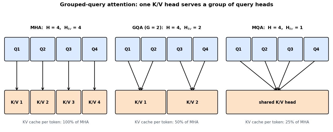
Three panels each showing four query head boxes above their key/value heads: MHA has four separate KV heads, GQA with group size two has two KV heads each fed by two query heads, and MQA has one KV head shared by all four query heads

Figure 1: The only structural change is how many distinct K/V heads exist; query heads are never merged, so each still has its own projection and its own attention pattern over the shared keys.

Mathematical Formulation:
$H_{kv} = H / G$
$g(i) = \lfloor i / G \rfloor$
$M_{tok} = 2 L H_{kv} d_h b$
$W_K^{(g)} = \frac{1}{G} \sum_{i \in \mathcal{G}_g} W_K^{(i)}$

Where:

$H$ is the number of query heads, $G$ the group size, and $H_{kv}$ the resulting number of key/value heads; $G = 1$ recovers MHA and $G = H$ recovers MQA.
$i \in \{0,\ldots,H-1\}$ indexes query heads and $g(i)$ is the KV head that head $i$ reads, so heads are assigned to groups by contiguous blocks.
$M_{tok}$ is the KV cache bytes per token, with $L$ layers, head dimension $d_h$ , bytes per element $b$ , and the factor 2 covering K and V; total cache is $M_{tok}$ times batch times sequence length.
$\mathcal{G}_g$ is the set of query-head indices in group $g$ , and the last line is the mean-pooling initialization used when converting an MHA checkpoint; the same averaging is applied to $W_V$ .

The payoff is easiest to see with a concrete configuration. A Llama-3-70B-shaped model has $L = 80$ , $H = 64$ , and $d_h = 128$ ; in FP16 that is 2.5 MiB per token of KV cache under MHA, 320 KiB under GQA with 8 KV heads, and 40 KiB under MQA. At a 32K context and batch size 1 those become 85.9 GB, 10.7 GB, and 1.34 GB. On a single H100 with 3.35 TB/s of HBM bandwidth, reading a 10.7 GB cache once costs roughly 3.2 ms per decoded token against roughly 26 ms for the 85.9 GB version; tensor parallelism divides both numbers, but the ratio is fixed by $H_{kv}$ and does not improve with more hardware. That freed memory is also what lets a server hold many more concurrent sequences, which is usually a larger throughput win than the per-token latency itself.

Log-scale bar chart of FP16 KV cache size at 32K context for a 70B-shaped model: MHA with 64 KV heads needs 85.9 GB, GQA with 8 KV heads needs 10.7 GB, and MQA with 1 KV head needs 1.34 GB, with a dashed line marking 80 GB of H100 HBM

Figure 2: FP16 KV cache for one 32K-token sequence on an 80-layer, 64-head, 128-dim model. Under MHA the cache alone would consume an entire 80 GB H100 before any weights are loaded.

Property	MHA	GQA (8 KV heads)	MQA
KV heads	64 (one per query head)	8 (group size 8)	1 (shared by all)
Cache per token (FP16)	2.5 MiB	320 KiB	40 KiB
Decode speed	Slowest, bandwidth bound on the cache	Close to MQA at long context	Fastest
Quality	Reference	Within noise of MHA on most benchmarks	Measurable drop, notably on long-input summarization
Tensor parallelism	Shards cleanly	Shards cleanly when $H_{kv}$ equals the shard count	KV must be replicated on every shard
Training stability	Stable baseline	Stable; uptrainable from an MHA checkpoint	Reported instability at scale

August 15, 2026