Category: Medium

DL0113 VLM Object Hallucination

Explain the primary causes of Object Hallucination in VLMs, for a captioning feature built on a model like LLaVA or Qwen2-VL.

Answer

Object hallucination is the case where a vision-language model asserts an object that is not present in the image, and it is not one bug but the sum of four largely independent failure sources stacked along the encode → project → decode pipeline. The vision tower is usually a frozen contrastively-trained ViT, so it encodes globally discriminative semantics and is measurably weak on small objects, counts, duplicates, and absence; the projector then compresses the image to a fixed budget of visual tokens (576 for CLIP ViT-L/14 at 336 px, only 32 query tokens for a BLIP-2 style Q-Former), discarding spatial detail the decoder can never recover. On the language side, the decoder was pretrained on text alone and carries a strong object co-occurrence prior, so whenever the visual evidence for a token is weak the prior decides: “dining table” pulls in “fork”, “kitchen” pulls in “refrigerator”. Instruction tuning makes this worse rather than better, because much visual SFT data is written by a text-only model from captions and bounding boxes and therefore contains ungrounded details, and the training objective rewards confident, fluent, detailed answers with no penalty term for an unsupported noun. Finally, decoding itself drifts: attention to visual tokens concentrates on a few early anchor positions and decays with sequence position, so late sentences are generated nearly blind, and once a wrong noun is emitted it conditions everything after it, producing the well-documented snowball effect.

(1) Weak Visual Features: a contrastive image-text objective optimizes for retrieval-level discrimination, not localization, so paired images differing in one small detail can receive nearly identical embeddings.
(2) Token And Resolution Budget: a fixed low-resolution grid plus projector compression means thin, small, or crowded objects arrive at the decoder as a few blurred features.
(3) Language Co-occurrence Prior: the text-pretrained decoder completes plausible scenes, and objects that frequently co-occur with the true content are the ones hallucinated first.
(4) Instruction Data Noise And Yes-Bias: SFT data generated from captions and boxes contains details never visible, and presence questions are answered affirmatively far more often than chance.
(5) Objective Mismatch: next-token cross-entropy has no grounding loss, and helpfulness-oriented preference tuning rewards verbosity, which mechanically increases the number of nouns at risk.
(6) Autoregressive Drift: visual attention mass decays over the generated sequence and hallucinated nouns become context, so error rate grows with output length rather than with model size.

Pipeline diagram: a 336 by 336 image enters a frozen ViT-L/14 encoder, a projector emits 576 visual tokens, a text-pretrained LLM decoder generates a caption, with four labelled causes attached to the encoder, projector, decoder, and the autoregressive feedback loop

Figure 1: Each stage can independently drop or overwrite visual evidence: the frozen contrastive encoder loses fine detail, the projector loses spatial resolution, the text-only prior fills the gap, and the sampling loop recycles its own mistakes.

The two benchmark families separate these causes reasonably well. CHAIR parses generated captions against a fixed object vocabulary and reports the fraction of mentioned objects that are absent, which makes drift visible because the metric worsens as captions get longer. POPE instead asks balanced yes/no presence questions and splits the negatives three ways: random objects, popular objects, and adversarial objects chosen because they co-occur most often with the ground-truth objects. The gap between the random and adversarial splits is close to a direct measurement of language-prior dominance, and the reported yes-ratios above 90% for several 2023-era models are a direct measurement of the SFT affirmation bias. A useful diagnostic in the same spirit is to score a candidate token twice, once with the image and once with the image removed, since a near-zero difference means the prior, not the pixels, chose that word.

Mathematical Formulation:
$s_t = \log p_\theta(y_t \mid v, x, y_{1:t-1})$
$s_t^{\mathrm{lang}} = \log p_\theta(y_t \mid x, y_{1:t-1})$
$\Delta_t = s_t - s_t^{\mathrm{lang}}$
$s_t^{\mathrm{cd}} = (1 + \alpha)\, s_t - \alpha\, s_t^{\mathrm{dist}}$
$\mathrm{CHAIR}_i = \frac{|H|}{|M|}$

Where:

$y_t$ is the token generated at step $t$ and $y_{1:t-1}$ the tokens already committed, which is why an early mistake is irreversible.
$v$ is the sequence of projected visual tokens (576 for a ViT-L/14 336 px grid, 32 for a Q-Former) and $x$ is the text prompt.
$s_t^{\mathrm{lang}}$ is the same score with the image dropped, so $\Delta_t$ is the visual grounding margin; $\Delta_t \approx 0$ means the token was chosen by the language prior alone.
$s_t^{\mathrm{dist}}$ is the score under a distorted or noised image and $\alpha \geq 0$ the contrast strength, giving the contrastive decoding adjustment used by VCD-style mitigations.
$M$ is the set of object mentions parsed from a caption and $H \subseteq M$ the subset absent from the annotation, so $\mathrm{CHAIR}_i$ is an instance-level hallucination rate in $[0, 1]$ .
Required condition for the margin test: both scores must be computed at the same step with identical $y_{1:t-1}$ , otherwise the two distributions are not comparable.

Two panel schematic chart: left panel shows attention mass on visual tokens declining from 0.30 to 0.06 across six generated sentence indices, right panel shows hallucinated object rate rising from 0.03 to 0.40 across the same indices

Figure 2: Schematic of the drift pattern reported by attention-analysis studies and by CHAIR-versus-length ablations: as generation proceeds, attention mass on visual tokens falls while the hallucinated-object rate rises, so long free-form captions hallucinate far more than short answers from the same model.

Aspect	Visual encoding bottleneck	Language prior dominance	Decoding-time drift
Typical symptom	Misses or confuses small, thin, or duplicated objects; counting and absence errors	Invents objects that usually co-occur with what is really there, such as a fork beside a dining table	First sentence accurate, later sentences increasingly invented; repeated nouns
Diagnostic probe	MMVP-style image pairs differing in one visual detail; linear probes on frozen features	POPE adversarial split versus random split; the grounding margin with and without the image	CHAIR plotted against caption length or max_new_tokens
Effect of a bigger decoder	Little help; the same weak features are described more confidently	Often worse, because a stronger text prior overrides weak visual evidence	Roughly unchanged; this is a sequence-length effect, not a capacity effect
Cheapest effective fix	Higher input resolution or dynamic tiling, more visual tokens, unfreezing the tower late in training	Contrastive decoding against a distorted image, plus preference tuning on grounded and ungrounded response pairs	Shorter outputs, beam-level over-trust penalties, post-hoc detector verification

August 17, 2026

DL0112 VLM Visual Grounding

How do VLMs perform Visual Grounding (predicting 2D/3D bounding boxes)?

Answer

Visual grounding asks the model to return the image region a phrase refers to, and current VLMs differ mainly in where the coordinates are physically produced. The dominant generalist recipe treats a box as text: coordinates are normalized and quantized onto a fixed grid (Kosmos-2 adds 1024 dedicated location tokens, Qwen-VL emits integers from 0 to 999 inside <box> markers, Qwen2.5-VL moved to absolute pixel values inside JSON) and the language model decodes them autoregressively under ordinary cross-entropy, so detection, referring expression comprehension, and grounded captioning all become one sequence task. The specialist recipe keeps a DETR-style decoder with learnable queries, a box regression head, and L1 plus GIoU losses, fusing text into the visual features and aligning region embeddings to word embeddings contrastively (MDETR, GLIP, Grounding DINO, Florence-2). A third, hybrid recipe uses an LLM hidden state as a prompt for an external mask or box decoder, as LISA does by feeding a <SEG> embedding to SAM. Whichever decoder is used, localization quality is mostly decided upstream: the connector has to hand the LLM patch tokens with their 2D layout and position information intact, at a resolution where the target object still covers several patches. 3D grounding extends the output to a 7 to 9 DoF box and introduces the real difficulty, depth and scale ambiguity, resolved either from point clouds (ScanRefer-style proposal-and-match pipelines) or monocularly with camera intrinsics, as in Cube-LLM.

(1) Coordinates As Text: a box becomes four discrete symbols on a normalized grid, so the only training signal is token cross-entropy, with no IoU-aware term and no set matching.
(2) The Connector Decides Localization: raster-ordered ViT patch tokens through an MLP projector preserve geometry, while abstractors that pool everything into a few dozen learned queries discard the spatial layout a box depends on.
(3) Resolution Beats Bin Count: quantization error at 1000 bins is sub-pixel, but a small object that occupies one patch cannot be localized tightly at any bin resolution, which is why dynamic resolution and tiling (AnyRes, Qwen2-VL M-RoPE) matter more than the tokenizer.
(4) Detection-Head Decoding: query-based decoders with region-word contrastive alignment still lead on tight-IoU metrics and emit hundreds of boxes in a single forward pass.
(5) Hidden State As Prompt: a referent or <SEG> token embedding can drive SAM or a 3D mask decoder, decoupling language reasoning from pixel-level decoding.
(6) 3D Adds Scale, Not Just Dimensions: monocular predictions are only consistent if camera intrinsics enter the model or the normalization, otherwise depth estimates do not transfer across datasets.
(7) Metrics And Supervision: RefCOCO family Acc@0.5 for 2D, [email protected] on ScanRefer for 3D, and every box target must be expressed in the same resized or tiled frame the encoder sees.

Diagram of a vision language model grounding pipeline: image, ViT encoder, MLP projector, LLM decoder, and three output paths producing location tokens, a referent hidden state for SAM or a DETR box head, and a 3D head using camera intrinsics

Figure 1: One shared perception stack, three places to produce coordinates. The path image → ViT patches → projector → LLM is identical; only the last stage differs, and the projector is where grounding is usually won or lost.

It is worth doing the arithmetic on the tokenizer, because interviewers often assume quantization is the limiting factor. With a 1000-bin normalized grid on a 1344 px side, the worst-case error per edge is about 0.67 px, far below what Acc@0.5 can detect. The real sensitivity is object size: a square object of side $s$ whose four edges each shift by $d$ has $\mathrm{IoU} = (s-d)^2 / (2s^2 - (s-d)^2)$ , so a 16 px object falls below 0.5 IoU once edges move about 3 px, while a 128 px object tolerates roughly 24 px. That is why generalist grounding scores jumped with higher effective input resolution rather than with finer coordinate grids: the earliest text-token generalists sat near 52 Acc@0.5 on RefCOCO val, Qwen-VL reached roughly 89, and Florence-2-L about 93, close to dedicated grounding detectors.

Mathematical Formulation:
$t_k = \mathrm{round}\left(\frac{c_k}{S}(n-1)\right)$
$p(b \mid I, q) = \prod_{k=1}^{4} p(t_k \mid I, q, t_{1:k-1})$
$\epsilon_{\max} = \frac{S}{2(n-1)}$
$\epsilon_{\max} = \frac{1344}{2 \cdot 999} \approx 0.67$
$\mathcal{L}_{\mathrm{box}} = \lambda_1 \lVert b - \hat{b} \rVert_1 + \lambda_2 (1 - \mathrm{GIoU})$
$B_{3D} = (x, y, z, w, h, l, \theta)$
$(u, v, 1)^{\top} = \frac{1}{z} K (x, y, z)^{\top}$

Where:

$b = (c_1, c_2, c_3, c_4)$ is the target box in the encoder’s resized pixel frame of side $S$ , and $\hat{b}$ is the prediction.
$t_k$ is the $k$ -th coordinate token and $n$ the number of bins (1024 for Kosmos-2 location tokens, 1000 for Qwen-VL integers).
$I$ is the image, $q$ the referring expression, and $t_{1:k-1}$ the previously emitted coordinate tokens, so decoding is strictly autoregressive.
$\epsilon_{\max}$ is the worst-case quantization error per edge in pixels, which scales linearly with input side and inversely with bin count.
$\lambda_1, \lambda_2$ weight the L1 and GIoU terms used by regression-head decoders; text-token models have no analogue of either.
$B_{3D}$ is a 3D box with center $(x, y, z)$ , extents $(w, h, l)$ , and yaw $\theta$ ; full 9 DoF variants add pitch and roll.
$K$ is the camera intrinsic matrix and $(u, v)$ the projected image point; this constraint is the required initial condition for monocular 3D grounding, since without $K$ the depth $z$ and the extents trade off freely.

Two panel chart: left panel shows worst-case per-edge quantization error in pixels versus number of coordinate bins for 448, 1344 and 3840 pixel inputs on log axes; right panel shows IoU versus per-edge shift in pixels for 16, 32 and 128 pixel objects with an IoU equals 0.5 threshold line

Figure 2: Left: a 1000-bin grid costs well under one pixel per edge even at high resolution, so coordinate tokenization is rarely the bottleneck. Right: the Acc@0.5 budget is roughly 3 px of edge error for a 16 px object, 6 px for 32 px, and 24 px for 128 px, which is why small-object grounding is an effective-resolution problem.

Property	Coordinates as text tokens (Kosmos-2, Qwen-VL)	Detection-head decoding (MDETR, Grounding DINO, Florence-2)	Hidden state as decoder prompt (LISA, Grounded 3D-LLM)
Where coordinates appear	In the text stream, as quantized or absolute numbers inside markers or JSON	From query embeddings in a cross-modal decoder with an explicit box head	Implicitly: a referent token embedding conditions an external mask or box decoder
Training signal	Token cross-entropy only, no IoU term	L1 plus GIoU with Hungarian matching, plus region-word contrastive alignment	Mask or box loss backpropagated into the LLM through the prompt embedding
Multi-instance output	Costs about 4 to 8 decoded tokens per box, so dense scenes are slow	Hundreds of boxes in one parallel forward pass	One region per referent token; needs several tokens for several targets
Strength	Unifies grounding with dialogue, counting, OCR, and grounded captioning in one head	Best tight-IoU accuracy and recall under a fixed latency budget	Pixel-accurate masks and 3D shapes without teaching the LLM geometry
Typical failure	Hallucinated coordinates for absent objects, plus parse failures and no calibrated confidence	Weak compositional or relational language, since reasoning capacity is limited	Two-stage error coupling; the frozen decoder caps achievable boundary quality

August 17, 2026

DL0110 VLM Image-Text Token Alignment

How do you align image tokens with text tokens in a vision-language model, for example in a system like LLaVA or Qwen2-VL?

Answer

Alignment is not one operation but three that have to agree: a representation map, a sequence layout, and a training curriculum. The dominant recipe runs a frozen contrastive vision encoder over the image, then a small trainable connector projects every patch embedding into the LLM’s token embedding space so the image becomes a block of ordinary tokens occupying real sequence positions. A CLIP ViT-L/14 at $336 \times 336$ produces $24 \times 24 = 576$ patch embeddings of width 1024, and a two-layer MLP maps them to the LLM width (4096 for a 7B decoder); the tokenizer’s single image placeholder is expanded in place into those 576 vectors. From that point alignment is learned by plain next-token prediction: text tokens read image positions through the same causal self-attention, and the gradient of the caption loss is what teaches the connector which visual direction means “a red bus”. The competing topology keeps images out of the sequence entirely and injects them through gated cross-attention layers inserted into a frozen LLM, as in Flamingo and Llama 3.2 Vision, trading sequence length for extra parameters.

(1) Shared Embedding Space: the connector’s only job is to land visual features in the same $d_{\text{model}}$ -dimensional space the token embedding table lives in, which is why an MLP with roughly 20M parameters is enough.
(2) Placeholder Expansion: the prompt carries one image placeholder id, and at embedding time that row is replaced by the $N$ projected vectors, so nothing downstream of the embedding layer knows the difference.
(3) Positional Alignment: patches are flattened row-major, so a purely 1D RoPE makes a vertical neighbor 24 positions away; 2D or multimodal RoPE restores height and width structure explicitly.
(4) Two Injection Topologies: prefix tokens with full self-attention are simple and preserve fine detail; gated cross-attention keeps the text stream’s length untouched and protects text-only ability.
(5) Staged Curriculum: stage 1 tunes only the connector on image-caption pairs with a frozen encoder and LLM, then stage 2 unfreezes the LLM on instruction data.
(6) Token Budget Is The Real Constraint: prefill attention is $O(L^2)$ in total sequence length, so pixel unshuffle, learned query resamplers, and tiling policies exist purely to control $N$ .

Pipeline diagram: a 336 by 336 image is encoded by a frozen ViT-L/14 into 576 patch features of width 1024, an MLP connector projects them to 4096 dimensions, and the resulting image tokens are spliced into the LLM token sequence between text embeddings before a causal decoder stack

Figure 1: The connector is the only trainable component in stage 1; after projection the 576 image tokens are indistinguishable from text embeddings to the decoder, which fuses both streams in a single causal self-attention stack.

Two details decide whether the alignment survives at scale. The first is resolution: a fixed $336 \times 336$ view destroys the small text and thin structures that document and chart questions depend on, so production models either tile the image into crops plus a downscaled thumbnail (AnyRes) or feed native resolution with a variable token count. The second is cost: because prefill attention grows quadratically, an AnyRes scheme with four crops plus a thumbnail spends 2,880 image tokens and roughly 25x the attention work of one 576-token view, before a single text token is generated. Compression is the usual answer, either a $2 \times 2$ pixel unshuffle that folds four patches into one channel-concatenated token or a query-based resampler that squeezes any number of patches into 32 or 64 learned slots. Both save compute by throwing away exactly the spatial precision that grounding and OCR need, which is why token budget, not connector architecture, is where most VLM design arguments actually land.

Mathematical Formulation:
$Z_v = g_{\phi}(x_{\text{img}})$
$H_v = W_2\,\sigma(W_1 Z_v)$
$N = \frac{H W}{P^2 r^2}$
$N = \frac{336 \cdot 336}{14^2 \cdot 1} = 576$
$E = [\, e(t_{1:k}),\; H_v,\; e(t_{k+1:m}) \,]$
$\mathcal{L} = -\sum_{i} \log p_{\theta}(t_i \mid t_{1:i-1}, H_v)$

Where:

$x_{\text{img}}$ is the image and $g_{\phi}$ the frozen vision encoder, giving patch features $Z_v \in \mathbb{R}^{N \times d_v}$ with $d_v = 1024$ for ViT-L.
$W_1, W_2$ and the nonlinearity $\sigma$ form the MLP connector, producing $H_v \in \mathbb{R}^{N \times d_{\text{model}}}$ in the LLM embedding space.
$H, W$ are image height and width, $P$ the patch size, and $r$ the pixel-unshuffle factor ( $r = 1$ means no merging, $r = 2$ cuts tokens 4x).
$e(\cdot)$ is the text embedding lookup, $t_{1:m}$ the prompt and response tokens, and $k$ the position of the image placeholder that $H_v$ replaces.
$E$ is the assembled input of length $L = m + N - 1$ , and $\mathcal{L}$ is the autoregressive loss masked to response tokens only, so no loss is computed on image positions.
Required initial condition: $g_{\phi}$ must already be language-aligned (CLIP or SigLIP pretraining), otherwise stage 1 has to learn the semantics as well as the projection.

Bar chart of image token counts and relative prefill attention cost for four vision-language configurations: 576 tokens at 1x, 1280 tokens at 4.9x, 1536 tokens at 7.1x, and 2880 tokens at 25x

Figure 2: Higher-resolution alignment policies buy detail with sequence length, and since prefill attention is $O(L^2)$ , moving from a single 576-token view to a five-crop AnyRes layout costs about 25x the attention work per prompt.

Property	MLP connector (prefix tokens)	Query resampler (Q-Former, Perceiver)	Gated cross-attention
Where fusion happens	In the input sequence, before layer 1	In the connector, then in the input sequence	Inside the decoder, at interleaved new layers
Tokens added to the LLM sequence	One per patch, 576 to 2,880 typical	Fixed, 32 to 64 regardless of resolution	Zero
New parameters	Smallest, roughly 20M for a 7B model	Moderate, a small transformer plus queries	Largest, extra attention plus tanh gates in the decoder
Prefill and KV-cache cost	Grows quadratically with token count	Nearly flat in image resolution	Linear in image features, no text-side growth
Typical failure mode	Latency and context blowup on multi-image or video prompts	Information bottleneck: weak OCR, dense counting, fine grounding	Harder to train, weaker at precise pixel-level reference
Text-only ability	Can regress once the LLM is unfrozen	Same risk if the LLM is tuned	Preserved by construction with a frozen LLM and zero-init gates

August 17, 2026

DL0106 Stable Diffusion Architecture

Explain the key components of the Stable Diffusion architecture and how they interact during image generation.

Answer

Stable Diffusion is three separately trained networks plus one training-free sampler, and only one of the three is trained on the diffusion objective. A frozen KL-regularized VAE maps a $512 \times 512 \times 3$ image to a $64 \times 64 \times 4$ latent and back; a frozen CLIP text encoder turns the prompt into a $77 \times 768$ sequence of token embeddings; and a conditional U-Net (860M parameters in SD 1.5) predicts the noise present in a noisy latent, given the timestep and the text context. At generation time the sampler starts from $z_T \sim \mathcal{N}(0, I)$ on the latent grid and repeats a fixed loop: call the U-Net, combine the conditional and unconditional predictions with classifier-free guidance, then let the scheduler (DDIM, Euler, DPM-Solver) take one step of the reverse process. After 20 to 50 such steps the VAE decoder is called exactly once to turn the final latent into pixels, so the full path is encode → denoise → decode with the text encoder feeding every denoising step through cross-attention.

(1) VAE Codec: a convolutional encoder and decoder pair, frozen after stage-one training with an L1 plus LPIPS plus patch-GAN objective, that removes imperceptible high-frequency detail so the denoiser works on 16,384 values instead of 786,432.
(2) Text Encoder: CLIP ViT-L/14’s transformer, frozen, producing per-token hidden states rather than a single pooled vector, which is what makes word-level prompt control possible.
(3) U-Net Denoiser: the only trained diffusion component, built from ResBlocks that receive a sinusoidal timestep embedding through a learned projection added to their feature maps, interleaved with transformer blocks.
(4) Cross-Attention Is The Conditioning Interface: queries come from the latent feature map, keys and values come from the text context, so the prompt influences the image at 16 separate points in SD 1.5’s U-Net.
(5) Scheduler: not a network at all but a numerical solver for the reverse SDE or probability-flow ODE, which is why you can swap samplers and step counts on a trained checkpoint without retraining.
(6) Classifier-Free Guidance: each step runs the U-Net twice, once with the prompt and once with the empty string, and extrapolates between them, which doubles the per-step cost and is the main knob for prompt adherence.

Block diagram of Stable Diffusion generation: a text prompt enters a frozen CLIP text encoder producing a 77 by 768 context that feeds cross-attention in the U-Net denoiser; starting from Gaussian noise in a 64 by 64 by 4 latent, the U-Net output passes through classifier-free guidance and a scheduler step, loops for 20 to 50 steps, and the final latent is decoded once by the frozen VAE decoder into a 512 by 512 image

Figure 1: The loop is the architecture. The U-Net is evaluated twice per step for guidance, the text encoder runs once for the whole generation, and the decoder runs once at the end; everything inside the loop stays on the small latent grid.

Inside the U-Net the latent descends a resolution ladder, $64 \rightarrow 32 \rightarrow 16 \rightarrow 8$ , with channel widths 320, 640, 1280, 1280, and climbs back up with skip concatenations from the matching encoder level. Attention is deliberately not applied everywhere: in SD 1.5 the transformer blocks sit at the $64$ , $32$ , and $16$ levels plus the mid block, and the deepest $8 \times 8$ level is pure convolution, because self-attention cost grows as $O(N^2)$ in the token count and the highest-resolution level already carries 4,096 tokens. SDXL rebalances exactly this: it drops attention at the finest level entirely and stacks far more transformer blocks at $32$ and $16$ , which is how it reaches 2.6B parameters while remaining trainable at $1024 \times 1024$ . Each transformer block is self-attention, then cross-attention, then a GEGLU feed-forward, so spatial coherence and prompt alignment are handled by two different mechanisms in the same block.

U-shaped diagram of the SD 1.5 denoiser: four downsampling levels at 64 by 64 with 320 channels, 32 by 32 with 640, 16 by 16 with 1280 and 8 by 8 with 1280, a mid block with attention, and four upsampling levels, with dashed skip-concatenation links between matching levels and attention marked at the top three levels and the mid block only

Figure 2: The SD 1.5 U-Net applies self-attention and cross-attention at three of four resolutions and leaves the deepest $8 \times 8$ level convolution-only; skip concatenations carry high-frequency structure past the bottleneck so the decoder path can restore fine detail.

Mathematical Formulation:
$z_T \sim \mathcal{N}(0, I)$
$Q = W_Q\,\varphi(z_t)$
$K = W_K\,\tau(y)$
$V = W_V\,\tau(y)$
$\mathrm{Attn} = \mathrm{softmax}\!\left(\frac{QK^{\top}}{\sqrt{d}}\right)V$
$\hat{\epsilon}_t = \epsilon_u + s\,(\epsilon_c - \epsilon_u)$
$z_{t-1} = \mathrm{Step}(z_t, \hat{\epsilon}_t, t)$
$\hat{x} = \mathcal{D}(z_0 / s_z)$

Where:

$z_t \in \mathbb{R}^{64 \times 64 \times 4}$ is the latent at timestep $t$ , and $\hat{x}$ is the decoded image.
$\varphi(z_t)$ is the flattened spatial feature map entering a transformer block, and $\tau(y)$ is the frozen CLIP context of shape $77 \times 768$ .
$W_Q, W_K, W_V$ are the per-layer projections and $d$ is the head dimension; queries carry image content while keys and values carry text.
$\epsilon_c = \epsilon_\theta(z_t, t, \tau(y))$ and $\epsilon_u = \epsilon_\theta(z_t, t, \tau(\varnothing))$ are the conditional and unconditional noise predictions, and $s$ is the guidance scale (typically $5 \leq s \leq 9$ ).
$\mathrm{Step}$ is the scheduler update (DDIM, Euler, DPM-Solver), applied for $t$ descending over the chosen 20 to 50 timesteps.
$\mathcal{D}$ is the frozen VAE decoder and $s_z = 0.18215$ the latent scaling constant; the required initial condition is $z_T \sim \mathcal{N}(0, I)$ , which only holds because $s_z$ normalizes the latent variance.

Component	SD 1.5	SDXL	SD3 / Flux
Latent codec	KL-VAE, f = 8, 4 channels, about 84M parameters	Retrained f = 8 VAE, still 4 channels	f = 8 VAE widened to 16 channels
Text encoder	CLIP ViT-L/14, 77 x 768 context	CLIP ViT-L plus OpenCLIP ViT-bigG, concatenated to 77 x 2048 plus a pooled vector	CLIP-L, CLIP-G and T5-XXL, giving long-prompt and typography understanding
Denoiser	U-Net, 860M, attention at 64, 32 and 16	U-Net, 2.6B, no attention at the finest level, deep transformer stacks at 32 and 16	MMDiT transformer, 2B to 12B, no convolutional U-Net at all
Conditioning path	Cross-attention in 16 transformer blocks	Cross-attention plus pooled text, original size and crop coordinates added to the timestep embedding	Joint self-attention over concatenated text and image tokens, with separate weights per modality
Objective and native resolution	Epsilon-prediction, 512 x 512	Epsilon-prediction base with a v-prediction refiner, 1024 x 1024	Rectified flow matching, 1024 x 1024 with multi-aspect buckets

August 17, 2026

DL0105 DiT: Diffusion Transformers

What is the core architectural innovation of Diffusion Transformers (DiT) compared to traditional U-Net-based diffusion models?

Answer

The core innovation is mostly subtractive: DiT deletes the multi-scale convolutional U-Net and replaces it with a plain ViT-style transformer that runs on a flat sequence of latent patch tokens at constant resolution and constant width, with no downsampling, no upsampling, and no encoder-decoder skip connections. A $32 \times 32 \times 4$ latent from an 8x VAE is cut into non-overlapping $p \times p$ patches ( $p = 2$ gives 256 tokens), linearly projected to width $d$ , given positional embeddings, and pushed through $N$ identical blocks. The only diffusion-specific machinery left is how conditioning enters: adaLN-Zero regresses a per-block scale, shift, and residual gate from the summed timestep and class embeddings, with the gate initialized to zero so each block starts as an identity map. Because the backbone is isotropic, sample quality becomes a smooth function of transformer Gflops rather than of hand-tuned channel schedules, and DiT-XL/2 (28 blocks, width 1152, 675M parameters, 118.6 Gflops) reached FID 2.27 with classifier-free guidance on ImageNet $256 \times 256$ after 7M training steps, ahead of the U-Net LDM and ADM baselines. That predictable scaling, plus the ability to reuse ordinary transformer infrastructure, is why later systems such as Stable Diffusion 3 and video generators adopted DiT-style backbones.

(1) Isotropic Token Stack: patchify once, then keep the sequence length and hidden width fixed through every block, so there is no multi-scale hierarchy and no skip connections to carry high-frequency detail.
(2) adaLN-Zero Conditioning: timestep and class are injected by modulating LayerNorm and gating the residual branch instead of through cross-attention or extra input channels, and the zero-initialized gate makes a 28-block stack start as the identity.
(3) Patch Size Is A Compute Knob: halving $p$ quadruples the token count and roughly quadruples backbone Gflops without adding parameters, which makes compute and capacity independently tunable.
(4) Quality Tracks Gflops: FID decreases monotonically with backbone Gflops across model sizes and patch sizes, so a smaller model with small patches can beat a larger model with large patches.
(5) Infrastructure Reuse: the backbone is a standard transformer, so FlashAttention, sequence and tensor parallelism, and spatiotemporal patching for video all transfer directly from the LLM and ViT ecosystem.

Side-by-side diagram: on the left a U-Net with three encoder ResBlocks descending in resolution, a mid block, three upsampling decoder blocks and dashed skip connections; on the right a DiT stack of patchify, 28 DiT blocks with adaLN-Zero conditioning, and a final linear unpatchify layer

Figure 1: The U-Net spends parameters on a resolution pyramid with skip connections, while DiT keeps one token sequence at fixed width and pushes all conditioning through adaLN-Zero modulation of each block.

The conditioning choice was not incidental. The DiT paper ablated four options at matched compute: in-context conditioning (append timestep and class as extra tokens), cross-attention to a two-token condition sequence, plain adaptive LayerNorm, and adaLN-Zero. The ranking was consistent, with adaLN-Zero best, then adaLN, then cross-attention, then in-context, and adaLN-Zero also added the fewest Gflops because it needs no extra tokens or extra attention operation. The zero-initialized gate matters because a deep residual stack whose blocks all start as identity behaves like a shallow network early in training, which is the same trick that stabilizes very deep ResNets and ViTs. The cost of dropping skip connections is that all high-frequency reconstruction has to be learned inside the token stack and by the VAE decoder, which is one reason DiT operates in a compressed latent space rather than on raw pixels.

Mathematical Formulation:
$T = \frac{H}{p} \cdot \frac{W}{p}$
$c = \mathrm{emb}(t) + \mathrm{emb}(y)$
$(\gamma_i, \beta_i, \alpha_i) = \mathrm{MLP}_i(c)$
$\hat{z} = (1 + \gamma_1)\,\mathrm{LN}(z) + \beta_1$
$z \leftarrow z + \alpha_1\,\mathrm{MSA}(\hat{z})$
$\mathcal{C}_{\mathrm{attn}} = O(T^2 d)$

Where:

$T$ is the token count after patchifying a latent of spatial size $H \times W$ with patch size $p$ ; for $H = W = 32$ and $p = 2$ this gives $T = 256$ .
$c$ is the pooled conditioning vector built from the diffusion timestep $t$ and the class or text embedding $y$ .
$\gamma_i, \beta_i$ are the scale and shift applied to the normalized activations of sub-layer $i$ , and $\alpha_i$ is the residual gate; $i \in \{1, 2\}$ indexes the attention and feed-forward sub-layers.
$z \in \mathbb{R}^{T \times d}$ is the token sequence, $\mathrm{LN}$ is LayerNorm without learnable affine parameters, and $\mathrm{MSA}$ is multi-head self-attention (the feed-forward sub-layer uses $\gamma_2, \beta_2, \alpha_2$ identically).
$\mathcal{C}_{\mathrm{attn}}$ is the per-layer attention cost, quadratic in $T$ and therefore quartic in the inverse patch size.
Required initial condition: $\alpha_1 = \alpha_2 = 0$ at step 0, so every block is an identity map and the residual stream passes through unchanged.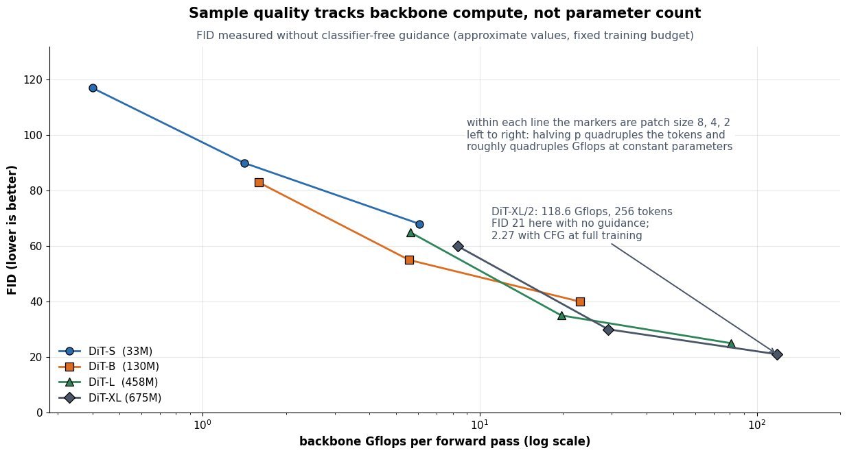

Log-x line chart of FID against backbone Gflops for DiT-S, DiT-B, DiT-L and DiT-XL, each line connecting patch sizes 8, 4 and 2, showing FID falling monotonically as Gflops rise

Figure 2: Approximate FID against backbone Gflops at a fixed 400K-step training budget and without classifier-free guidance, which is why the absolute values sit far above the guided FID 2.27 quoted for the fully trained DiT-XL/2. What matters here is the trend: quality tracks compute rather than parameter count, so DiT-B with $p = 2$ can outrun DiT-L with $p = 8$ despite having far fewer parameters.

Property	DiT	U-Net (ADM, LDM, SDXL)
Spatial handling	One fixed-length token sequence, no resampling and no skips	Resolution pyramid 32 → 16 → 8 → 4 → 8 → 16 → 32 with skip connections
Conditioning path	adaLN-Zero: per-block scale, shift, and zero-initialized residual gate from $c$	Timestep embedding added inside ResBlocks, text or class via cross-attention
Compute knobs	Depth, width, and patch size; patch size changes Gflops at constant parameters	Channel multipliers, blocks per level, and which levels get attention
Inductive bias	Minimal beyond positional embeddings, so it needs more data and compute to pay off	Strong locality and multi-scale bias, sample-efficient at small budgets
Cost as resolution grows	$O(T^2 d)$ attention, so latent compression and patch size are load-bearing	Convolutions grow linearly in pixels; attention only at low-resolution levels
Scaling behavior	FID a smooth decreasing function of Gflops, easy to extrapolate	Gains depend on hand-designed schedules and saturate less predictably

One caveat when quoting numbers in an interview: FID is only comparable within a fixed evaluation protocol. The headline 2.27 comes from the fully trained DiT-XL/2 sampled with classifier-free guidance at scale 1.5; the same checkpoint sampled without guidance lands near 9.6, and the scaling sweep above uses a much shorter 400K-step budget with no guidance at all. Guidance, training steps, sampler, and step count all move the number by more than the architectural gap being discussed, so state the protocol alongside the score.

August 16, 2026

DL0103 Stable Diffusion Latent Space

What is latent diffusion, and why does Stable Diffusion run diffusion in a VAE latent space?

Answer

Latent diffusion splits image generation into two stages that are trained separately: a convolutional autoencoder first compresses pixels into a small spatial latent, and the diffusion model then learns the noise process entirely inside that latent grid. Stable Diffusion uses a KL-regularized VAE with downsampling factor $f = 8$ , so a $512 \times 512 \times 3$ image becomes a $64 \times 64 \times 4$ latent: 786,432 values collapse to 16,384, a 48x reduction in the tensor the U-Net has to denoise. The motivation is that the two stages solve different problems. Pixel-space diffusion wastes most of its capacity and most of its training steps modeling imperceptible high-frequency detail, exactly the information a perceptual codec throws away for free; the autoencoder handles that perceptual compression once, and the diffusion model is left with the semantic compression problem of arranging layout, objects, and style. The compute argument is even stronger than the 48x suggests, because the U-Net contains self-attention: token count drops from 262,144 to 4,096, so any $O(N^2)$ attention block gets $f^4 = 4096$ times cheaper. That is what turned high-resolution text-to-image training from a large-cluster project into something reproducible on modest hardware, and what makes 50-step sampling on a consumer GPU feasible at all.

(1) Two-Stage Factorization: the autoencoder is trained first and then frozen; the diffusion model never sees a pixel, and the decoder is invoked exactly once at the end of sampling.
(2) Quadratic Savings On Attention: the latent grid has $f^2$ fewer positions, so convolutions get $f^2$ cheaper and self-attention gets roughly $f^4$ cheaper.
(3) It Is Not A Generative VAE: the KL weight is tiny (on the order of $10^{-6}$ ) and the reconstruction loss adds LPIPS plus a patch discriminator, so the encoder behaves as a sharp lossy codec rather than a prior you would ever sample from.
(4) Latent Scaling Matters: encoder outputs are multiplied by a constant (0.18215 for SD 1.x, 0.13025 for SDXL) so the latent has roughly unit variance and the standard noise schedule reaches a true $\mathcal{N}(0, I)$ terminal state.
(5) Cheap Conditioning And Editing: CLIP text embeddings enter through cross-attention at every latent resolution, and img2img, inpainting, and ControlNet all operate on the same small latent grid.
(6) The Decoder Is The Fidelity Ceiling: nothing the diffusion model does can recover detail the 4-channel latent discarded, which is why small text, fine textures, and tiny faces degrade first.

Pipeline diagram: a 512 by 512 by 3 image enters a VAE encoder producing a 64 by 64 by 4 latent, an iterative denoising U-Net conditioned by CLIP text cross-attention operates on the latent for T steps, and a VAE decoder maps the result back to pixels

Figure 1: Training and sampling both live in the 4,096-token latent grid; the frozen encoder and decoder are the only components that ever touch the 262,144-pixel image, and text conditioning enters the denoiser through cross-attention.

The choice of $f$ is a genuine trade-off rather than a free win. The original LDM ablations show that $f \in \{4, 8\}$ is the sweet spot: at $f = 1$ or $2$ training is slow because the model is still doing perceptual compression itself, while at $f = 32$ with only 4 channels the autoencoder becomes the bottleneck and sample quality saturates no matter how long the diffusion model trains. Channel count $c$ is the other lever, and it is the one that later models moved: SD3 and Flux keep $f = 8$ but raise the latent to 16 channels, quartering the compression ratio from 48 to 12 to trade a little step cost for a much better reconstruction ceiling on text and fine structure. A practical consequence of the frozen-codec design is that latents are model-specific: an SDXL latent decoded by an SD 1.5 decoder produces color-shifted garbage, because the two autoencoders were trained with different scaling and channel statistics.

Mathematical Formulation:
$z_0 = s \cdot \mathcal{E}(x)$
$\hat{x} = \mathcal{D}(z_0 / s)$
$z_t = \sqrt{\bar\alpha_t}\, z_0 + \sqrt{1 - \bar\alpha_t}\, \epsilon$
$\mathcal{L} = \mathbb{E}\left[\lVert \epsilon - \epsilon_\theta(z_t, t, \tau(y)) \rVert_2^2\right]$
$\rho = \frac{3 f^2}{c}$
$\rho = \frac{3 \cdot 64}{4} = 48$

Where:

$x \in \mathbb{R}^{H \times W \times 3}$ is the image and $\hat{x}$ its reconstruction; $z_0 \in \mathbb{R}^{h \times w \times c}$ is the clean latent with $h = H/f$ and $w = W/f$ .
$\mathcal{E}$ and $\mathcal{D}$ are the frozen VAE encoder and decoder, and $s$ is the latent scaling constant that normalizes the variance.
$t \in \{1, \ldots, T\}$ is the timestep, $\bar\alpha_t$ the cumulative noise schedule, and $\epsilon \sim \mathcal{N}(0, I)$ the sampled Gaussian noise.
$\epsilon_\theta$ is the latent denoiser (U-Net in SD 1.x and SDXL, a transformer in DiT-style successors), and $\tau(y)$ is the text-encoder output injected by cross-attention.
$f$ is the spatial downsampling factor and $c$ the latent channel count; $\rho$ is the element compression ratio, which is 48 for $f = 8, c = 4$ and 12 for $c = 16$ .
Required initial condition at sampling: $z_T \sim \mathcal{N}(0, I)$ on the latent grid, which only holds if $s$ was applied and $\bar\alpha_T \approx 0$ .

Log-scale bar chart of self-attention cost reduction relative to pixel space at 512 by 512 resolution: factor 1 for pixel space with 262144 tokens, 256 for f equals 4, 4096 for f equals 8, and 65536 for f equals 16

Figure 2: Because self-attention scales as $O(N^2)$ in the token count, compressing by $f$ cuts attention cost by $f^4$ ; the $f = 8$ setting used by Stable Diffusion buys a 4096x reduction while keeping the decoder’s reconstruction error acceptable.

Property	Latent diffusion (Stable Diffusion)	Single-stage pixel diffusion	Cascaded pixel diffusion
Where noise is added	A 64x64x4 VAE latent	Directly on RGB pixels at full resolution	Pixels at 64×64, then two super-resolution diffusion stages
Denoiser input size at 512×512	4,096 tokens, 16,384 values	262,144 tokens, 786,432 values	4,096 tokens in the base model, full resolution in the last upsampler
Training and sampling cost	Lowest; one model, attention roughly 4096x cheaper per block	Highest; attention is usually dropped or windowed to stay tractable	Moderate but multiplied by the number of stages
Fidelity ceiling	Bounded by decoder reconstruction error, independent of training length	No codec bottleneck; exact pixel modeling is possible	No codec bottleneck, but upsamplers can hallucinate detail
Typical failure mode	Mangled small text, smeared fine texture, artifacts on tiny faces	Under-trained global structure for a fixed compute budget	Error accumulation and train/test mismatch between stages

August 16, 2026

DL0100 GAN Framework

Explain the GAN framework: what are the two networks optimizing, and why does the generator learn anything at all?

Answer

A Generative Adversarial Network trains two networks against each other. The generator $G$ maps a latent noise vector $z \sim p_z$ (typically $\mathcal{N}(0, I)$ ) to a sample in data space, and the discriminator $D$ outputs the probability that its input came from the real dataset rather than from $G$ . They share one value function in a two-player minimax game: $D$ maximizes the log-likelihood of correctly classifying real and fake batches, while $G$ minimizes the same quantity, so the generator’s only learning signal is the gradient that flows backward through the discriminator into the fake samples. The theory is clean: for a fixed $G$ the optimal discriminator is the density ratio $p_{data}/(p_{data} + p_g)$ , and substituting it turns the generator’s objective into the Jensen-Shannon divergence between the data distribution and the model distribution, uniquely minimized when $p_g = p_{data}$ . The practical payoff is that $G$ is an implicit model: it never evaluates a likelihood, it just produces a sample in one forward pass, which is why GANs remain attractive whenever sampling latency matters.

(1) Two Networks One Objective: there is a single value function $V(D,G)$ ; the discriminator ascends it and the generator descends it, so no explicit reconstruction or likelihood term is ever written down.
(2) Discriminator As A Density Ratio: the optimal $D^*$ encodes $p_{data}(x)/p_g(x)$ , which is exactly the information the generator needs about where it is over- or under-producing mass.
(3) Implicit Sampling Model: $p_g$ is defined only through the pushforward of $p_z$ by $G$ , so sampling is a single forward pass but density evaluation is impossible.
(4) Non-Saturating Generator Loss: the theoretical $\log(1 - D(G(z)))$ term has almost no gradient while the generator is bad, so implementations maximize $\log D(G(z))$ instead.
(5) Alternating Updates, No Loss Curve To Read: training alternates discriminator and generator steps and seeks a saddle point, not a minimum, so a falling loss means nothing and quality is judged with FID or human inspection.

Diagram of the GAN framework: latent noise feeds the generator which produces fake samples, real samples and fake samples both feed the discriminator which outputs a probability of being real, and a dashed path carries the generator gradient back from the discriminator output into the generator

Figure 1: The generator never sees a real sample directly; it only receives gradient that has been routed backward through the discriminator, which is why the quality of $D$ bounds what $G$ can learn.

A training step draws a minibatch of real samples and a minibatch of latents, updates $D$ on both, then updates $G$ with $D$ held fixed. The original paper allowed $k$ discriminator steps per generator step; almost everyone now uses $k = 1$ and controls the balance with regularization instead. The three interventions that matter most in practice are spectral normalization or an R1 gradient penalty to keep the discriminator smooth, two-timescale learning rates so the discriminator can stay slightly ahead, and an exponential moving average of the generator weights for evaluation. The classic failure modes are mode collapse, where $G$ concentrates on a few outputs that currently fool $D$ , and vanishing generator gradient, where a discriminator with near-perfect separation returns almost nothing useful.

Mathematical Formulation:
$\min_G \max_D V(D, G)$
$V(D,G) = \mathbb{E}_{x \sim p_{data}}[\log D(x)]$
$\quad + \mathbb{E}_{z \sim p_z}[\log (1 - D(G(z)))]$
$D^*(x) = \frac{p_{data}(x)}{p_{data}(x) + p_g(x)}$
$C(G) = 2 \, \mathrm{JSD}(p_{data} \, \| \, p_g) - \log 4$
$\mathcal{L}_G = -\mathbb{E}_{z \sim p_z}[\log D(G(z))]$

Where:

$V(D,G)$ is the shared value function, maximized by $D$ and minimized by $G$ .
$x \sim p_{data}$ is a real sample and $z \sim p_z$ a latent vector, so $G(z)$ is a generated sample and $D(\cdot) \in (0,1)$ is the estimated probability of being real.
$p_g$ is the implicit distribution induced by pushing $p_z$ through $G$ ; it is never evaluated, only sampled.
$D^*$ is the optimal discriminator for a fixed $G$ , and $C(G) = \max_D V(D,G)$ is the resulting generator criterion; $\mathrm{JSD}$ is the Jensen-Shannon divergence, so $C(G) \geq -\log 4$ with equality only at $p_g = p_{data}$ .
$\mathcal{L}_G$ is the non-saturating generator loss actually used in code; it shares the same fixed point as the minimax form but has large gradient when $D(G(z))$ is near 0, which is the required starting condition of training.

Log-scale plot of generator gradient magnitude versus the discriminator score on fake samples, showing the saturating loss curve one over one minus D staying near one at low scores while the non-saturating curve one over D rises to one hundred

Figure 2: Gradient magnitude of the two generator losses with respect to $D(G(z))$ . At the start of training the discriminator wins easily, the saturating form contributes almost nothing, and the non-saturating form is roughly 100x larger at a score of 0.01.

Property	GAN	VAE	Diffusion
Training objective	Adversarial minimax, no likelihood term	ELBO, a lower bound on log-likelihood	Weighted denoising regression on noised inputs
Sampling cost	One forward pass through the generator	One forward pass through the decoder	20 to 1000 network evaluations unless distilled
Sample sharpness	Very sharp, no pixel-averaging term to blur output	Typically blurry from the reconstruction term	Very sharp, current state of the art on text-to-image
Mode coverage	Weakest; mode collapse is the signature failure	Good coverage, over-smoothed samples	Good coverage from a likelihood-style objective
Training stability	Saddle-point game, needs penalties and careful balance	Single stable objective	Single stable objective, scales predictably

August 16, 2026

DL0099 Masked Autoencoding MAE

What is masked autoencoding (MAE, or masked language modeling) as a representation learning objective?

Answer

Masked autoencoding is a denoising self-supervised objective: hide a random subset of the input units, then train the network to reconstruct exactly what was hidden from the surviving context. The supervision is free because the labels are the withheld input itself, and the representation quality comes from the fact that reconstruction cannot be solved by copying: predicting a masked word or a masked image region requires the encoder to carry semantic, long-range context in its hidden states. BERT-style masked language modeling is the discrete version, masking about 15% of tokens and predicting a softmax over the vocabulary at those positions. MAE is the continuous vision version, masking about 75% of image patches and regressing raw pixels with an asymmetric encoder-decoder: a deep ViT encoder that only ever sees the visible 25% of patches, plus a shallow decoder that is discarded after pretraining. That asymmetry is what makes it cheap, and it scales: a ViT-Huge pretrained with MAE on ImageNet-1K alone reaches 87.8% top-1 after fine-tuning, with over 3x faster pretraining than a full-token baseline.

(1) Masking Manufactures The Labels: no annotation is required, so the objective scales with raw data; the only design decisions are what to mask, how much, and what target to regress or classify.
(2) Asymmetric Encoder-Decoder: the encoder processes only unmasked tokens and mask tokens enter at the decoder, so both compute and the pretrain-finetune input mismatch shrink dramatically.
(3) Masking Ratio Tracks Information Density: text is dense and semantic so 15% suffices, while adjacent pixels are highly redundant and need 75% before the task stops being local interpolation.
(4) The Target Defines The Representation: raw pixels, per-patch normalized pixels, discrete VQ tokens (BEiT), or latent teacher features (data2vec) all train the same encoder toward different levels of abstraction.
(5) Strong Fine-Tuning, Weak Linear Probing: MAE features are highly non-linear, so they beat contrastive methods after fine-tuning but lag them under a frozen linear probe or k-NN retrieval.

Flow diagram of the MAE pipeline: a 4 by 4 patch grid with 75 percent of cells masked, an arrow into a ViT encoder that processes only the 49 visible tokens, then a block that inserts mask tokens and restores order, then a lightweight 8-block decoder, then the reconstructed patch grid

Figure 1: The MAE pipeline for a ViT-L/16 at 224 pixels: of 196 patches only 49 reach the encoder, mask tokens are inserted just before a shallow decoder, and the MSE loss is computed on masked patches only.

Two details separate the text and vision instantiations. BERT cannot drop masked positions because the prediction head must sit at those positions, so the literal [MASK] symbol is fed to the encoder during pretraining and never appears at fine-tuning time; the original recipe patches this discrepancy by replacing only 80% of selected tokens with [MASK], 10% with a random token, and leaving 10% unchanged. MAE removes the problem structurally: masked patches are simply deleted from the encoder’s input sequence, and the mask token is a learned vector injected at the decoder. The second detail is the loss support. Computing the reconstruction error on masked patches only matters, since including visible patches lets the model spend capacity on an identity mapping and measurably hurts downstream accuracy.

Mathematical Formulation:
$\mathcal{L}_{\mathrm{MLM}} = -\sum_{i \in \mathcal{M}} \log p_{\theta}(x_i \mid \tilde{x})$
$\hat{x} = D\big(E(x_{\mathcal{V}}), m\big)$
$\mathcal{L}_{\mathrm{MAE}} = \frac{1}{|\mathcal{M}|} \sum_{i \in \mathcal{M}} \|\hat{x}_i - x_i\|_2^2$
$|\mathcal{V}| = (1 - \rho)\,N$
$C_{\mathrm{attn}}(\mathcal{V}) / C_{\mathrm{attn}}(N) = (1 - \rho)^2$

Where:

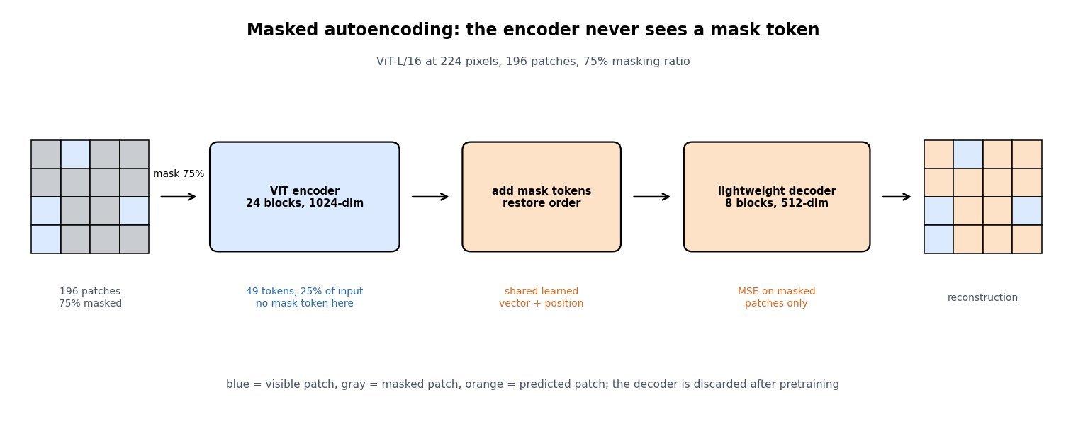
$\mathcal{L}_{\mathrm{MLM}}$ is the cross-entropy over masked token positions and $\mathcal{L}_{\mathrm{MAE}}$ the per-patch MSE; both are averaged over masked positions only.
$x_i$ is the true content at position $i$ , $\hat{x}_i$ the prediction, and $\tilde{x}$ the corrupted sequence containing $\texttt{[MASK]}$ symbols.
$\mathcal{M}$ and $\mathcal{V}$ are the masked and visible index sets, disjoint with $|\mathcal{M}| + |\mathcal{V}| = N$ for $N$ total tokens or patches.
$E$ is the deep encoder applied to visible tokens alone, $D$ the shallow decoder, and $m$ the shared learned mask-token embedding plus positional encoding.
$\rho$ is the masking ratio: $\rho = 0.15$ for BERT and $\rho = 0.75$ for MAE, giving $|\mathcal{V}| = 49$ of $N = 196$ patches.
$C_{\mathrm{attn}}$ is quadratic self-attention cost, so at $\rho = 0.75$ encoder attention drops to $1/16$ and the token-wise MLP cost to $1/4$ ; targets are usually per-patch normalized pixels rather than raw values.

Line chart of ImageNet top-1 accuracy against masking ratio from 10 to 90 percent, showing a nearly flat fine-tuning curve near 85 percent and a strongly peaked linear-probing curve rising to about 73.5 percent at a 75 percent masking ratio then falling sharply at 90 percent

Figure 2: Approximate ViT-L behaviour versus masking ratio: fine-tuning is nearly flat from 40% to 80%, while linear probing peaks sharply near 75%, which is why a ratio that looks extreme for text is the vision default.

Property	MAE (pixel targets)	MLM (BERT-style)	Contrastive / joint embedding
Corruption level	75% of patches removed	15% of tokens replaced or kept	No masking; two augmented views
Encoder input	Visible tokens only, no mask token	Full sequence including [MASK]	Full clean views
Prediction head	8-block 512-dim decoder, discarded	Single linear layer over the vocabulary	MLP projector plus temperature
Best transfer mode	Full fine-tuning and dense tasks	Fine-tuning on token-level tasks	Frozen features, k-NN, zero-shot retrieval
Main weakness	Capacity spent on high-frequency detail; weak linear probe	Only ~15% of positions produce gradient per step	Augmentation-sensitive; risk of collapse

August 16, 2026

DL0094 Evaluating an LLM

How do you evaluate an LLM?

Answer

There is no single number, so I treat evaluation as a stack of layers chosen to match how the model will actually be used: intrinsic likelihood (perplexity or bits per byte) at the bottom, static capability benchmarks above it, automated graders such as unit tests and LLM-as-judge, human pairwise preference, and finally an online A/B test on the real product metric. Each layer up the stack is closer to user value and more expensive, so cheap layers act as fast regression gates and expensive layers make ship decisions. The practical work is defining the task metric first, then building a private evaluation set drawn from production traffic, because public leaderboards measure a distribution that is rarely yours. Three things decide whether an evaluation is worth anything: contamination control, judge calibration against human labels, and error bars. Most reported “improvements” of one or two points on a 1000-item benchmark are inside the noise band and would not survive a paired significance test.

(1) Start From The Deployment Task: a RAG assistant is scored on groundedness, citation precision, and refusal correctness, a coding model on pass@k against hidden tests, an agent on end-to-end task completion; a generic leaderboard score answers none of these.
(2) Intrinsic Versus Extrinsic: perplexity is cheap and useful for pretraining and quantization regressions, but it is not comparable across tokenizers and correlates weakly with instruction-following quality.
(3) Static Benchmarks Decay: MMLU-Pro, GPQA, MATH, HumanEval, and SWE-bench Verified are reproducible and cheap, but they saturate and they leak into pretraining corpora, so contamination checks (n-gram overlap, held-out variants, release-date filtering) are mandatory.
(4) Automated Graders Scale, With Bias: the loop is sample responses → grade with a rubric or unit tests → aggregate with intervals; a judge model shows position, verbosity, and self-preference bias, so swap the answer order and calibrate agreement with humans before trusting it.
(5) Human Preference Is The Open-Ended Gold Standard: pairwise votes fitted with a Bradley-Terry (Elo) model give a single latent quality score, at the cost of slow turnaround and annotator disagreement.
(6) Report Uncertainty, Safety, And Cost: every score needs a confidence interval and a paired test against the baseline, plus a separate axis for jailbreak resistance, toxicity, PII leakage, and the p95 latency and cost per request that decide whether the win is affordable.

Five stacked layers of LLM evaluation from intrinsic perplexity at the bottom through static benchmarks, automated graders, human preference, and production A/B testing at the top, with cost and fidelity increasing upward

Figure 1: The evaluation stack. Cheap layers at the bottom run on every commit as regression gates; the expensive layers at the top are the only ones that measure user value, so a release decision needs evidence from both ends.

Two failure modes dominate real evaluation work. The first is contamination: a model that has memorized a benchmark scores high without generalizing, which you detect by rewriting items into paraphrases or numeric variants and watching the score collapse, or by using benchmarks whose items post-date the training cutoff. The second is judge miscalibration: an LLM judge that prefers longer, more confidently worded answers will happily rank a verbose model above a correct one, so I always measure judge-human agreement (Cohen’s kappa above roughly 0.6 before the judge is allowed to gate a release) and control for response length. On top of that, generation is stochastic, so a benchmark run at temperature 0.7 has run-to-run variance of its own; fix seeds and decoding parameters, or report the mean over several runs. Finally, offline wins must be confirmed online, because the production metric that matters (resolution rate, edit distance to the accepted answer, escalation rate) frequently moves in the opposite direction from a benchmark score.

Property	Static benchmark	LLM-as-judge	Human preference
What it measures	Closed-form correctness on a fixed item set	Rubric compliance and pairwise win rate on open-ended prompts	Latent quality as perceived by real users or experts
Turnaround per model	Minutes to hours, fully automated	Hours, bounded by judge API throughput and cost	Days to weeks, bounded by annotator supply
Main failure mode	Contamination and saturation; near-zero headroom on old suites	Position, verbosity, and self-preference bias	Annotator disagreement and prompt-mix drift
Reproducible	Yes, if decoding and prompt template are pinned	Only against a pinned judge version; judge upgrades shift scores	No, each round is a fresh sample of raters
Best used for	CI regression gates and capability screening	Scaling open-ended comparison between candidate checkpoints	Final ranking and calibrating the automated judge

Mathematical Formulation:
$\mathrm{PPL} = \exp\left(-\frac{1}{T}\sum_{t=1}^{T}\log p(x_t \mid x_{1:t-1})\right)$
$\mathrm{pass@}k = 1 - \frac{\binom{n-c}{k}}{\binom{n}{k}}$
$P(a \succ b) = \frac{1}{1 + 10^{(R_b - R_a)/400}}$
$\mathrm{SE} = \sqrt{\frac{\hat{p}(1-\hat{p})}{N}}$

Where:

$\mathrm{PPL}$ is perplexity over a held-out sequence $x_1,\ldots,x_T$ , with $t$ indexing tokens; it depends on the tokenizer, so bits per byte is the cross-model comparable form.
$n$ is the number of samples drawn per coding problem, $c$ the number that pass the hidden tests, and $k$ the budget of attempts scored; this is the unbiased pass@k estimator, averaged over problems.
$P(a \succ b)$ is the modelled probability that response $a$ beats $b$ , and $R_a, R_b$ are the fitted Bradley-Terry ratings on the Elo scale, where a 100-point gap implies about a 64% win rate.
$\hat{p}$ is the observed accuracy on $N$ independent items and $\mathrm{SE}$ its standard error; the 95% interval is $\hat{p} \pm 1.96\,\mathrm{SE}$ , which for $\hat{p}=0.7$ and $N=1000$ is roughly $\pm 2.8$ points.
Required condition: items must be independent and not contaminated; when two models are scored on the same items, use a paired test (McNemar or a paired bootstrap) rather than comparing two independent intervals.

Bar chart of three model accuracies of 71.2, 73.5 and 78.9 percent on a 1000-item benchmark with 95 percent confidence interval error bars of about 2.8 points, showing the first two intervals overlapping

Figure 2: Accuracy with 95% intervals on a 1000-item benchmark. The 2.3-point gap between the first two models sits well inside the noise band, so an unpaired claim of improvement is unsupported; only the third model separates cleanly.

August 16, 2026

DL0093 Distillation vs Serving

When is distilling a large model into a small one a better strategy than serving the large model directly, for example behind a high-traffic assistant API?

Answer

Distillation wins when the recurring cost of inference, multiplied by sustained traffic, dominates the one-time cost of teacher labeling plus student training, and when the task distribution is narrow enough that the teacher’s surplus capability is never exercised. The decision is a break-even calculation: if the teacher costs $2.00 per 1k requests and an 8B student costs $0.25, and distillation costs $1,400 once (500k teacher-labeled prompts at $1,000 plus 200 GPU-hours at $400), the crossover is 800k requests, roughly 18 hours at 12 QPS. Two other conditions make distillation the only option rather than the cheapest one: a hard latency SLO that no batching strategy can meet with a 70B decoder, and a fixed memory envelope such as a phone NPU or a single 24 GB GPU, where quantization alone cannot close a 10x parameter gap. Serve the large model directly when traffic is low, when the input distribution is open-ended, or when the win is available more cheaply through quantization, speculative decoding, prompt caching, or a small-to-large cascade, since those preserve behavior and skip a new eval and re-qualification cycle. Distillation also carries a maintenance tax: every teacher upgrade reopens the labeling job, and the student inherits the teacher’s errors without the capacity to recover from them.

(1) Break-Even Volume: divide the one-time distillation cost by the per-request savings; below that volume, serving the teacher is strictly cheaper, and the payback period, not the compression ratio, is the number that decides the project.
(2) Latency Floor, Not Throughput: autoregressive decoding is memory-bandwidth bound and sequential, so per-token latency scales with parameter count and cannot be batched away; shrinking the model is one of the few levers that moves p99 rather than QPS per GPU.
(3) Task Breadth Decides Feasibility: on a stable, narrow task a student 8x smaller typically recovers 98-99% of teacher quality, while an open-ended assistant distribution loses many points because the teacher’s broad competence is exactly what is being compressed away.
(4) Hard Deployment Constraints: on-device, air-gapped, or offline targets impose a memory and power budget that no serving trick satisfies, so distillation becomes a requirement rather than an optimization.
(5) Cheaper Alternatives First: speculative decoding is distribution-preserving and needs no re-qualification, quantization is a one-line config change, and a router that sends easy traffic to a small model keeps the teacher available for the tail; distillation is the only lever that actually reduces the footprint, and it is the most expensive to maintain.

Mathematical Formulation:
$Q^{*} = \frac{C_{0}}{c_{L} - c_{S}}$
$C_{0} = N c_{L} + C_{\text{train}}$
$\mathcal{L} = (1-\lambda)\mathcal{L}_{\text{CE}} + \lambda \tau^{2} \mathcal{L}_{\text{KD}}$
$\mathcal{L}_{\text{KD}} = \mathrm{KL}(p^{T}_{\tau} \| p^{S}_{\tau})$

Where:

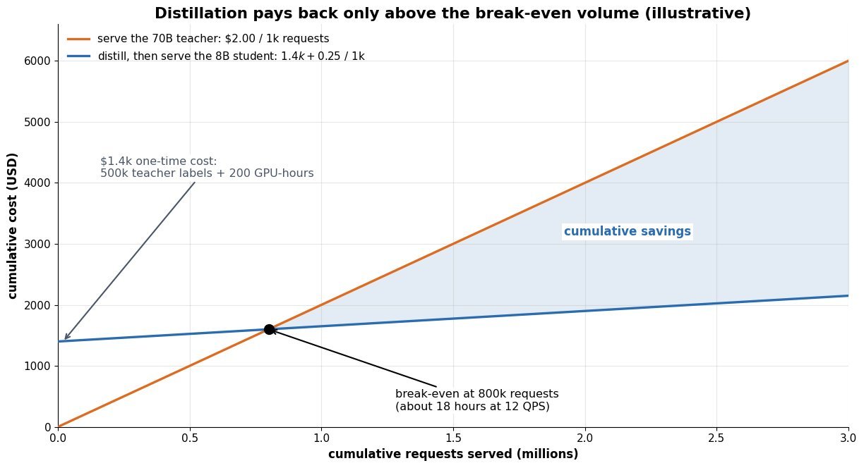
$Q^{*}$ is the break-even request volume, the point at which cumulative distilled-serving cost equals cumulative teacher-serving cost.
$c_{L}$ and $c_{S}$ are the marginal serving costs per request for the large teacher and the small student; the difference $c_{L} - c_{S}$ must be positive for distillation to ever pay back.
$C_{0}$ is the one-time cost, composed of teacher inference over $N$ unlabeled prompts plus student training $C_{\text{train}}$ ; engineering and eval time belong here too and usually exceed the compute.
$\mathcal{L}$ is the student objective, mixing hard-label cross-entropy $\mathcal{L}_{\text{CE}}$ with the distillation term $\mathcal{L}_{\text{KD}}$ under mixing weight $\lambda \in [0,1]$ .
$\tau$ is the softmax temperature applied to both teacher and student logits, and the $\tau^{2}$ factor rescales the gradient so $\lambda$ stays meaningful as $\tau$ changes; $p^{T}_{\tau}$ and $p^{S}_{\tau}$ are the tempered teacher and student distributions.
Required condition for the whole strategy: the student must also satisfy the latency and memory constraints, $t_{S} \leq \text{SLO}$ and $m_{S} \leq m_{\max}$ , which no amount of traffic volume can buy.

Line chart of cumulative serving cost in dollars against cumulative requests in millions: serving the 70B teacher rises linearly at 2 dollars per thousand requests from the origin, while the distillation path starts at 1400 dollars and rises at 0.25 dollars per thousand, crossing at 800 thousand requests with the savings region shaded beyond the crossing

Figure 1: Illustrative cost curves: the distilled path carries a $1.4k fixed intercept but an eight-times shallower slope, so the break-even sits at 800k requests and every request after that is pure savings.

The break-even math is only valid if the student actually holds quality on the traffic you will receive, and that depends far more on task breadth than on the compression ratio. A single-intent classifier, a fixed extraction schema, or one product domain compresses well because the teacher’s decision boundary in that slice is simple and you can generate unlimited soft targets for it; an open-ended assistant does not, because the surplus capacity is the product. When breadth is the problem, a cascade is usually the better answer than a bigger student: route every request to the distilled model, escalate the tail flagged by a confidence or verifier signal to the teacher, and you capture most of the cost win while keeping the quality ceiling. Whatever you choose, budget for the maintenance tax, since a teacher upgrade invalidates the student, drifting inputs silently move outside the distilled distribution, and you now own two eval suites instead of one.

Semi-log chart of percentage of teacher quality retained against student parameter count from 0.5B to 70B, showing a narrow single-domain task staying above the 98 percent floor from about 1B upward while an open-ended assistant task falls to roughly 71 percent at 1B and only reaches the floor near 20B

Figure 2: Illustrative quality retention: on a narrow task a 1B student already clears a 98% floor, while the same student on open-ended traffic gives up roughly 27 points, which is why breadth, not the compression factor, gates the decision.

Property	Distill to a small student	Serve large + quantization	Serve large + speculative decoding
Memory footprint	8-20x smaller, can drop from 8 GPUs to 1 or to a phone	2-4x smaller weights, KV cache mostly unchanged	Slightly larger, the drafter is an extra resident model
Quality guarantee	None, must be re-measured per task; tail regressions are common	Small measurable drift, worse at 4-bit and on long context	Distribution-preserving, output matches the teacher exactly
Typical latency gain	4-6x on per-token latency, the largest available lever	1.5-2.5x, bounded by bandwidth saved on weights	2-3x at low batch, degrades as batch size grows
One-time cost	Label generation, training runs, a new eval harness	Calibration pass plus a quality spot-check	Serving-stack work, no retraining of the target model
Cost when the teacher is upgraded	Full re-distillation and re-qualification	Re-run calibration only	Swap the target, optionally refresh the drafter
Wins when	High sustained traffic, narrow task, or a fixed device budget	You need a fast, low-risk cost cut on broad traffic	Latency matters, batches are small, and quality cannot move

August 16, 2026