Category: Medium

DL0074 GRU vs LSTM

How does a GRU differ from an LSTM, and when would you prefer one over the other?

Answer

Both are gated recurrent cells that replace the vanilla RNN’s repeated multiplication by an additive state update, which is what keeps gradients alive across long sequences. The LSTM carries two state tensors (the cell state $c_t$ and the hidden state $h_t$ ) and three gates: forget, input, and output. The GRU is a leaner reparameterization that keeps one state: it merges forget and input into a single update gate $z_t$ whose two branches are tied as $z_t$ and $1 - z_t$ , deletes the output gate so the full state is exposed to the next layer, and adds a reset gate $r_t$ that suppresses the previous state inside the candidate. The practical consequence is three weight blocks instead of four, so roughly 25% fewer recurrent parameters and matmuls per step, plus one less tensor to carry and initialize. Accuracy is usually close (Chung et al. 2014; Greff et al. 2017), so the choice is driven by data size, latency, and whether the task needs the LSTM’s unbounded memory.

(1) Gate Inventory: LSTM has forget, input, and output gates; the GRU has update and reset only, because tying the write and erase decisions into $z_t$ and $1 - z_t$ removes one gate and dropping the output gate removes another.
(2) One State vs Two: the LSTM’s protected cell state $c_t$ is never squashed on the recurrent path and is only revealed through the output gate, while the GRU’s single $h_t$ is both the memory and the emitted representation.
(3) Parameter and Compute Ratio: with input width $D$ and hidden width $H$ , the GRU costs exactly $3/4$ of the LSTM’s recurrent parameters and per-step FLOPs, which matters most when the recurrent stack dominates the model.
(4) Expressivity Gap: at finite precision, the LSTM’s additive, unsquashed cell state can implement a genuine counter, whereas the GRU’s convex-combination update keeps the state inside $[-1,1]$ and can only approximate counting (Weiss et al. 2018).
(5) How to Choose: prefer the GRU for small or medium datasets, short-to-medium sequences, and tight latency or memory budgets; prefer the LSTM for long sequences, large corpora, and tasks that need precise long-horizon bookkeeping such as language modeling.

Two side-by-side cell diagrams: the LSTM panel shows a cell-state track with multiply and add operators fed by forget and input gates plus an output gate producing h_t; the GRU panel shows a single hidden-state track with an update gate feeding both branches and a reset gate feeding the candidate

Figure 1: The LSTM keeps a separate cell-state track written by forget and input gates and read out through an output gate; the GRU folds everything onto one hidden-state track, where the update gate supplies both mixing weights and the reset gate only conditions the candidate.

Mathematical Formulation:
$c_t = f_t \odot c_{t-1} + i_t \odot \tilde{c}_t$
$h_t = o_t \odot \tanh(c_t)$
$\tilde{h}_t = \tanh(W_h x_t + r_t \odot U_h h_{t-1} + b_h)$
$h_t = (1 - z_t) \odot \tilde{h}_t + z_t \odot h_{t-1}$
$P_{\mathrm{LSTM}} = 4(HD + H^2 + H)$
$P_{\mathrm{GRU}} = 3(HD + H^2 + H)$

Where:

$h_t$ is the hidden state emitted at step $t$ and $c_t$ the LSTM’s internal cell state; both start from zero at $t = 0$ .
$x_t$ is the input at step $t$ , with $D$ its width and $H$ the hidden width.
$f_t, i_t, o_t$ are the LSTM forget, input, and output gates and $\tilde{c}_t$ its candidate, each of the form $\sigma(Wx_t + Uh_{t-1} + b)$ (with $\tanh$ for the candidate).
$z_t$ and $r_t$ are the GRU update and reset gates, both sigmoid, and $\tilde{h}_t$ is its candidate state.
$\odot$ is the elementwise product, $\sigma$ the logistic sigmoid mapping to $(0,1)$ , and $W, U, b$ the input, recurrent, and bias parameters of one gate block.
$P$ counts recurrent-cell parameters only, so the ratio $P_{\mathrm{GRU}}/P_{\mathrm{LSTM}} = 3/4$ holds for any $D$ and $H$ .

Grouped bar chart on a log scale of recurrent parameter counts for hidden widths 128, 256, 512 and 1024 with input width equal to hidden width: LSTM bars are 0.13M, 0.53M, 2.10M and 8.39M while GRU bars are 0.10M, 0.39M, 1.57M and 6.29M

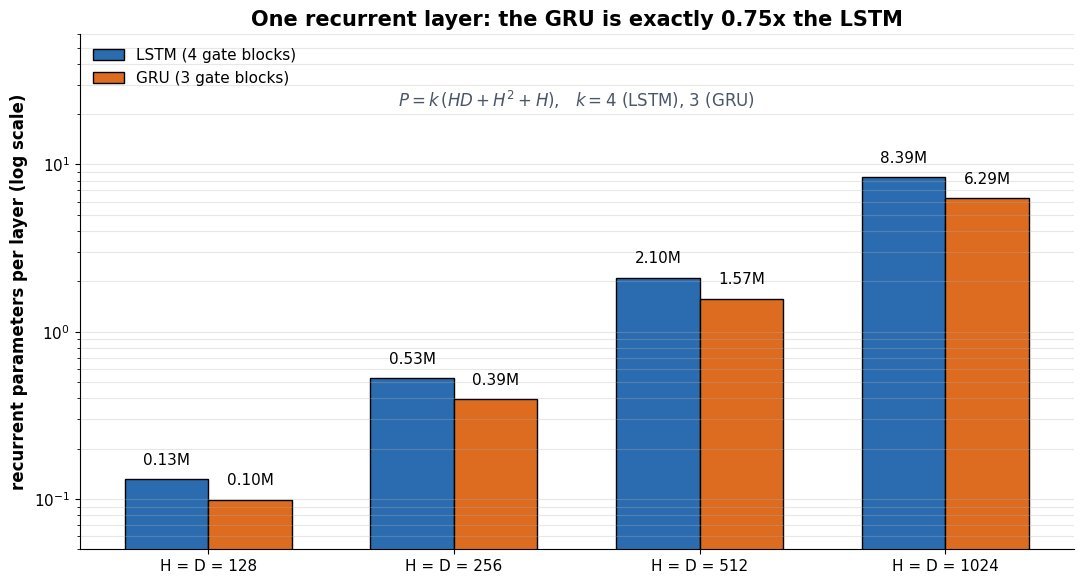
Figure 2: Recurrent parameters per layer with $D = H$ : three gate blocks instead of four give the GRU exactly 0.75x the LSTM count at every width, so at $H = 512$ one layer holds 1.57M against 2.10M.

Property	GRU	LSTM
Gates	2: update, reset	3: forget, input, output
State carried	Hidden state only	Hidden state plus cell state
Weight blocks	3	4
Params at D = H = 512	1.57M	2.10M
Memory exposure	Whole state is exposed downstream	Output gate filters what leaves the cell
Unbounded counting	No: state stays bounded by the convex update	Yes: additive, unsquashed cell state
Where it tends to win	Small data, short sequences, tight latency	Long sequences, large corpora, language modeling

August 14, 2026

DL0072 Inception Module

What is the Inception module, and how does it use parallel convolutions of different sizes?

Answer

The Inception module is the building block of GoogLeNet: instead of committing a layer to one kernel size, it runs several convolutional branches in parallel over the same input (1×1, 3×3, 5×5, plus a 3×3 max-pool path) and concatenates their outputs along the channel axis. Every branch uses stride 1 with padding chosen so all branches emit the same spatial size, which is what makes the concatenation legal. The naive form is prohibitively expensive because the 5×5 branch convolves over the full input depth, so the practical module inserts 1×1 convolutions as channel bottlenecks before the 3×3 and 5×5 convolutions and after the pooling path. The next layer therefore sees features at several receptive-field sizes at once, and the learned weights decide how much of each scale to use rather than the architect fixing one kernel per layer.

(1) Parallel Multi-Scale Branches: the 1×1, 3×3, 5×5, and pooling paths all read the identical input tensor, so one module covers several receptive fields; a face at 20 px and one at 60 px are both matched inside the same layer.
(2) Channel-Wise Concatenation: branches keep $H$ and $W$ identical (stride 1, pad 1 for 3×3, pad 2 for 5×5), and outputs are stacked on the channel dimension, so module output depth is the sum of branch depths, not their average.
(3) 1×1 Bottlenecks: convolution cost is linear in $C_{in} C_{out} k^2$ , so projecting 192 channels down to 16 before the 5×5 conv cuts that branch roughly 10x with a small accuracy cost.
(4) Dense Ops, Sparse Intent: the design approximates a sparse, locally-optimal connectivity structure using dense operations that BLAS and cuDNN execute efficiently, which is why GoogLeNet reached top ILSVRC-2014 accuracy at about 5M parameters, roughly 12x fewer than AlexNet.

Two side-by-side block diagrams of an Inception module: on the left the naive version sends the 28x28x192 input straight into 1x1, 3x3, 5x5 convolutions and a 3x3 max pool before filter concatenation; on the right the dimension-reduced version inserts 1x1 convolutions with 96 and 16 channels before the 3x3 and 5x5 convolutions and a 32-channel 1x1 projection after the pool

Figure 1: Naive versus dimension-reduced Inception module. The 1×1 convolutions shrink channel depth before the expensive kernels and project the pooled path, so concatenation does not grow depth without bound.

The pooling branch is the reason the naive module is unstable when stacked: max pooling preserves its input depth, so every module would add at least the full input depth back into the concatenated output and channel count would grow monotonically with depth. The 1×1 projection after the pool fixes this, and the same trick applied before the 3×3 and 5×5 convolutions is where nearly all the savings come from. Take the classic Inception (3a) block with a $28 \times 28 \times 192$ input and a 5×5 branch producing 32 maps.

Mathematical Formulation:
$y = \mathrm{concat}(y_1, y_3, y_5, y_p)$
$C = H_o W_o C_{out} k^2 C_{in}$
$C_{naive} = 28^2 \cdot 32 \cdot 5^2 \cdot 192 \approx 120 \times 10^6$
$C_{reduce} = 28^2 \cdot 16 \cdot 1^2 \cdot 192 \approx 2.4 \times 10^6$
$C_{conv} = 28^2 \cdot 32 \cdot 5^2 \cdot 16 \approx 10.0 \times 10^6$

Where:

$y_1, y_3, y_5, y_p$ are the outputs of the 1×1, 3×3, 5×5, and pooling branches, and $\mathrm{concat}$ stacks them on the channel axis, which requires all four to share the same $H_o \times W_o$ .
$C$ counts multiply-adds for one convolution, with $H_o W_o$ the output spatial size, $C_{in}$ and $C_{out}$ the input and output channels, and $k$ the kernel width.
$C_{naive}$ is the 5×5 branch applied to all 192 input channels; $C_{reduce}$ is the 1×1 projection to 16 channels and $C_{conv}$ the 5×5 conv on those 16, summing to about $12.4 \times 10^6$ , roughly a tenth of the naive branch.

Grouped bar chart of multiply-adds in millions per Inception 3a branch, naive versus dimension-reduced: 1x1 branch 9.6 and 9.6, 3x3 branch 173.4 and 101.2, 5x5 branch 120.4 and 12.4, pool branch 0 and 4.8, module total 303.5 and 128.0

Figure 2: Multiply-adds per branch for Inception (3a) on a $28 \times 28 \times 192$ input. The bottlenecks cut the 5×5 branch from about 120M to 12M and the module total from about 304M to 128M, while also shrinking output depth from 416 to 256 channels.

Branch	1×1 Reduction	Main Operation	Output Channels	Multiply-Adds
Point-wise	none needed	1×1 conv, 64 filters	64	9.6M
Medium scale	192 to 96	3×3 conv, 128 filters, pad 1	128	101.2M
Large scale	192 to 16	5×5 conv, 32 filters, pad 2	32	12.4M
Pooling	192 to 32, after the pool	3×3 max pool, stride 1, pad 1	32	4.8M
Concatenated	–	channel-axis concat, 28×28 preserved	256	128M

August 14, 2026

DL0071 VGG vs GoogLeNet vs ResNet

Compare VGG, GoogLeNet/Inception, and ResNet: what key problem did each architecture address?

Answer

The three architectures answer three different questions that the ImageNet era asked in sequence. VGG (2014) asked whether depth alone helps and showed that stacking small 3×3 convolutions to 16 or 19 weight layers beats wide shallow filters, but it paid for that with 138M parameters and 15.3 GFLOPs, roughly 90% of the parameters sitting in three fully connected layers. GoogLeNet/Inception (2014) asked how to get depth and multi-scale receptive fields cheaply: parallel 1×1, 3×3, 5×5, and pooling branches inside one Inception module, with 1×1 bottleneck convolutions cutting channel depth before the expensive kernels, plus global average pooling replacing the fully connected head, giving better accuracy than VGG with about 6.8M parameters and 1.5 GFLOPs. ResNet (2015) asked why depth stopped paying off past roughly 20 to 30 layers and identified the degradation problem: a 56-layer plain net reaches higher training error than a 20-layer one, so this is an optimization failure, not overfitting. Its fix, the identity shortcut $y = \mathcal{F}(x) + x$ , makes each block learn a residual and gives gradients a direct path, which made 152-layer and even 1000-layer networks trainable.

(1) VGG, Depth Through Uniformity: three stacked 3×3 layers match the 7×7 receptive field with fewer parameters and two extra nonlinearities, proving that a simple repeated motif scales; the cost is a parameter-heavy fully connected head and no answer to what happens beyond ~19 layers.
(2) Inception, Depth Under a Compute Budget: the module runs several kernel sizes in parallel so the network does not have to choose one scale per layer, and 1×1 reduce → 5×5 conv keeps the cost of the wide branches roughly an order of magnitude lower than the naive version.
(3) ResNet, Depth Without Degradation: residual blocks reframe the layer’s job as learning a correction to identity, so adding layers can never be worse than copying the input; combined with batch normalization and bottleneck blocks (1×1, 3×3, 1×1), it made very deep training routine.

Parameter Arithmetic:
$3 \times 3^2 C^2 = 27 C^2$
$1 \times 7^2 C^2 = 49 C^2$
$5^2 \cdot 192 \cdot 32 = 153{,}600$
$192 \cdot 16 + 5^2 \cdot 16 \cdot 32 = 15{,}872$

Where:

$C$ is the channel count held constant across the stack, so the first two lines compare three 3×3 layers against one 7×7 layer of identical receptive field: about 45% fewer weights and two extra ReLUs.
The third line is the naive Inception 5×5 branch: 192 input channels, 32 output channels, $5^2$ spatial taps.
The fourth line inserts a 1×1 reduce to 16 channels first, so the same branch costs 15,872 weights, roughly $10\times$ cheaper; this bottleneck is what let GoogLeNet run 22 layers at 1.5 GFLOPs.

Scatter plot of ImageNet top-5 error against parameter count on a log scale for VGG-16 at 138M parameters and 7.3 percent, GoogLeNet at 6.8M and 6.7 percent, ResNet-50 at 25.6M and 5.25 percent, and ResNet-152 at 60.2M and 4.49 percent

Figure 1: Accuracy did not come from parameter count: GoogLeNet beats VGG-16 with about $20\times$ fewer parameters, and ResNet improves again at moderate size. Evaluation protocols differ slightly across the original papers, so read the trend rather than the decimals.

The residual idea is the one that generalized furthest. Writing a block as $y = \mathcal{F}(x, \{W_i\}) + x$ means the optimizer only has to push $\mathcal{F}$ toward zero to recover the identity mapping, which is exactly the solution the deeper plain net failed to find. The gradient view is just as important: the identity term contributes an ungated path so the signal reaching early layers cannot vanish through repeated multiplication by small Jacobians. In practice the projection shortcut ( $1\times1$ convolution with stride 2) handles the stage boundaries where spatial size and channel count change.

Residual Formulation:
$y = \mathcal{F}(x, \{W_i\}) + x$
$\frac{\partial L}{\partial x} = \frac{\partial L}{\partial y}\left(I + \frac{\partial \mathcal{F}}{\partial x}\right)$

Where:

$x$ is the block input, $y$ its output, and $\mathcal{F}$ the two or three stacked convolutions with weights $\{W_i\}$ .
$I$ is the identity Jacobian of the shortcut; it keeps the gradient norm from collapsing even when $\partial \mathcal{F} / \partial x$ is tiny, which is why depth beyond 100 layers becomes trainable.
$L$ is the training loss; when shapes differ across a stage, $x$ is replaced by $W_s x$ with a projection shortcut.

Schematic training error curves over 160 epochs: a 56-layer plain network plateaus at a higher training error than a 20-layer plain network, while a 56-layer ResNet reaches the lowest training error

Figure 2: Schematic of the degradation problem: the deeper plain network settles at higher training error than the shallower one, ruling out overfitting; the residual version of the same depth trains to the lowest error.

Aspect	VGG (2014)	GoogLeNet / Inception (2014)	ResNet (2015)
Key problem addressed	Does depth with small kernels beat shallow wide kernels?	How to buy depth and multiple scales on a fixed compute budget	Degradation: deeper plain nets train worse
Signature component	Uniform 3×3 conv stacks plus 2×2 max pool	Inception module with 1×1 bottlenecks, global average pooling	Identity shortcut, bottleneck block (1×1, 3×3, 1×1), batch norm
Depth	16 or 19 weight layers	22 layers	18 to 152, and 1000+ in experiments
Parameters / compute	138M, 15.3 GFLOPs	~6.8M, 1.5 GFLOPs	25.6M, 3.8 GFLOPs (ResNet-50)
Main drawback	Huge FC head, memory hungry, stalls past ~19 layers	Hand-tuned, irregular module; harder to modify or scale	Still heavy for edge devices; deep variants give diminishing returns
Lasting legacy	3×3 as the default kernel; perceptual loss backbone	1×1 channel bottlenecks; no-FC classification heads	Residual connections in nearly every modern net, including Transformers

August 14, 2026

DL0069 RMSProp Adaptive Learning Rates

How does RMSProp adapt the learning rate per parameter?

Answer

RMSProp keeps a per-parameter exponential moving average of squared gradients and divides each gradient component by the square root of that average before stepping, so the effective learning rate shrinks for parameters with historically large gradients and grows for those with small or sparse ones. The running estimate $v_t$ acts as a per-coordinate normalizer: two parameters share one global learning rate yet move by very different amounts. On ill-conditioned surfaces, where curvature differs wildly across directions, this damps oscillation along steep directions while sustaining progress along shallow ones, something a single global learning rate cannot do. Tieleman and Hinton introduced the method in their 2012 Coursera lecture series to cope with non-stationary objectives such as mini-batch and recurrent training; Adam is essentially RMSProp plus a first-moment momentum term and bias correction.

(1) Per-Coordinate Normalization: each parameter steps by $\alpha\, g_t / (\sqrt{v_t} + \epsilon)$ ; a parameter whose gradients run 10x larger builds a 10x larger $\sqrt{v_t}$ , so its effective learning rate shrinks 10x and the two coordinates end up moving by comparable amounts instead of one dwarfing the other.
(2) Memory With a Window: the decay $\rho$ (0.9 in the original lecture; PyTorch’s RMSprop defaults to 0.99) makes $v_t$ an average over recent history, so the normalization adapts as the landscape changes instead of stalling like AdaGrad’s monotonically growing accumulator.
(3) No Bias Correction: $v_t$ starts at zero and is never corrected, so early steps are oversized; Adam fixes this with $\hat{v}_t = v_t / (1 - \rho^t)$ , one of the two additions (the other is momentum) that turn RMSProp into Adam.

Contour plot of the ravine f(x,y) = 0.05x^2 + 2y^2 with two 42-step trajectories from (-10, 4): the red SGD path zigzags across the steep y direction with decaying overshoots while creeping along x to about -1.5, and the blue RMSProp path settles into the valley without oscillating and travels along it to the minimum

Figure 1: On the ravine $f(x,y) = 0.05x^2 + 2y^2$ , SGD spends its budget oscillating across the steep $y$ direction and after 42 steps is still at $x \approx -1.5$ ; RMSProp normalizes both coordinates, never overshoots, and reaches $x \approx -0.3$ in the same 42 steps.

The same normalization explains RMSProp’s strength on sparse features. For an embedding row that receives a gradient only occasionally, $v_t$ decays toward zero between updates, so when a gradient finally arrives its effective learning rate $\alpha / \sqrt{v_t}$ is several times larger than a densely-updated parameter’s, and the rare signal is not drowned out by a global rate tuned for frequent gradients. The flip side appears at the start of every run: with $\rho = 0.99$ the first estimate is $v_1 = 0.01\, g_1^2$ , so the first step has magnitude $10\,\alpha$ whatever the gradient scale, a warmup-like quirk that Adam’s bias correction removes. In practice RMSProp remains a solid choice for RNNs and other non-stationary objectives, while vision recipes still often prefer well-tuned SGD with momentum for final generalization.

Two stacked panels over 60 training steps: top shows sqrt of v_t rising from 0.2 toward its asymptote of 2 for a parameter with large steady gradient while staying near 0.3 for a sparse-gradient parameter; bottom shows the effective learning rate alpha over sqrt(v_t) falling from 5 to 0.74 for the first parameter while the second stays near 2.9 in a sawtooth pattern

Figure 2: Two parameters over 60 steps with $\rho = 0.99$ : the one with a large steady gradient sees its effective learning rate $\alpha / \sqrt{v_t}$ fall 6.7x by step 60 (heading for $\alpha/2$ as $\sqrt{v_t} \to |g|$ ), while the sparse-gradient parameter still enjoys a roughly 4x larger rate.

Mathematical Formulation:
$v_t = \rho\, v_{t-1} + (1 - \rho)\, g_t^2$
$\theta_{t+1} = \theta_t - \frac{\alpha\, g_t}{\sqrt{v_t} + \epsilon}$

Where:

$g_t = \nabla f_t(\theta_t)$ is the minibatch gradient at step $t$ ; the squaring in the accumulator is element-wise.
$v_t$ is the per-parameter running average of squared gradients, with the same shape as $\theta$ , initialized to zero.
$\rho$ is the decay (0.9 in Hinton’s lecture, 0.99 by default in PyTorch), $\alpha$ the global learning rate, and $\epsilon \approx 10^{-8}$ a numerical floor guarding the division.
All operations are element-wise, so each parameter gets its own effective rate $\alpha / (\sqrt{v_t} + \epsilon)$ under one shared $\alpha$ .

Aspect	SGD + Momentum	RMSProp	Adam
State per Parameter	Velocity m (first moment)	Squared-gradient average v (second moment)	Both m and v
Normalization	None; one global rate for all coordinates	Gradient divided by sqrt(v) per coordinate	Bias-corrected m divided by sqrt(v-hat)
Early Steps	Stable from step one	Oversized; v underestimated with no correction	Bias correction keeps steps near alpha scale
Typical Strength	Final test accuracy on tuned vision recipes	RNNs and non-stationary objectives	Default for transformers and general use

August 12, 2026

DL0068 Computational Graphs

What is a computational graph, and why is it useful in deep learning frameworks?

Answer

A computational graph is a directed acyclic graph whose nodes are operations or stored values and whose edges are the tensors flowing between them. Deep learning frameworks materialize this graph while running the forward pass: PyTorch records it dynamically on every iteration (define-by-run), while early TensorFlow built the whole graph statically before execution. Its central use is reverse-mode automatic differentiation: every node carries a known local derivative, so the chain rule becomes a mechanical backward sweep that produces every parameter’s gradient in a single pass, whose cost is roughly 2-3 times the forward pass and does not grow with the number of parameters being differentiated. The same data structure also drives memory planning such as activation checkpointing, whole-graph compiler optimizations like kernel fusion in XLA or torch.compile, device placement, and deployment export to formats such as ONNX.

(1) Structure and Evaluation: nodes are ops or values and edges are tensors; the forward pass evaluates nodes in topological order and caches every intermediate, because the backward sweep needs those values to compute local derivatives.
(2) One Sweep, All Gradients: each node multiplies its incoming adjoint $\bar{v} = \partial L / \partial v$ by its local Jacobian and passes the result to its inputs, summing contributions at fan-out; a single reverse traversal yields gradients for all parameters, which is why backprop scales to billion-parameter models.
(3) Dynamic vs Static Graphs: PyTorch’s define-by-run graph follows arbitrary Python control flow and debugs like ordinary code; static graphs (TensorFlow 1, exported ONNX) trade that flexibility for ahead-of-time whole-graph optimization and portable deployment.

Forward computational graph of L = (wx + b - y)^2: input boxes x=2, w=3 feed a multiply node producing u=6, then an add node with b=1 producing z=7, a subtract node with y=5 producing e=2, and a square node producing L=4

Figure 1: Forward pass of $L = (wx + b - y)^2$ with $x=2,\ w=3,\ b=1,\ y=5$ : each op consumes its input tensors, emits one value, and caches it for the backward sweep.

The backward sweep traverses the same graph in reverse. Starting from the seed $\bar{L} = 1$ , each node applies the chain rule locally: the square node returns $2e = 4$ , the subtraction forwards $+4$ to $z$ and $-4$ to $y$ , the addition copies its adjoint to both $u$ and $b$ , and the multiplication swaps operands, delivering $\bar{w} = 4 \cdot x = 8$ and $\bar{x} = 4 \cdot w = 12$ . No node needs global knowledge of the loss; correctness of the whole sweep follows from composing local derivatives edge by edge. The figure shows $\bar{x}$ and $\bar{y}$ to make the mechanics uniform, but a framework skips those branches when the input and target carry requires_grad=False, so only $\bar{w}$ and $\bar{b}$ are actually materialized. When a value feeds several nodes (fan-out), its adjoint is the sum of the contributions along each outgoing edge, which is exactly the multivariate chain rule.

Backward pass over the same graph with arrows reversed: adjoint labels on every edge showing e-bar=4, z-bar=4, y-bar=-4, u-bar=4, b-bar=4, w-bar=4 times 2=8, x-bar=4 times 3=12, seeded by L-bar=1

Figure 2: The same graph in reverse: each node multiplies the incoming adjoint by its local derivative, so one sweep accumulates $\bar{w} = 8$ and $\bar{b} = 4$ at the leaves.

The graph pays for itself well beyond gradients. Since it records exactly which intermediates feed the loss, frameworks can plan memory: reverse mode must retain cached activations, so training a depth- $N$ network costs $O(N)$ activation memory, and gradient checkpointing cuts this to $O(\sqrt{N})$ by storing only boundary activations and recomputing each segment during the backward pass, at the price of roughly one extra forward evaluation. A static snapshot of the same graph lets compilers fuse ops, pick kernel layouts, and place tensors across devices, and exporters freeze it into a portable artifact. The trade-off is flexibility: a define-by-run graph is rebuilt every iteration, so data-dependent if-statements and loops simply work, while a static graph must capture control flow symbolically, which is why TensorFlow 2 defaulted to eager execution and recovers graph benefits selectively through tf.function tracing.

Mathematical Formulation:
$L = (w\,x + b - y)^2$
$\bar{v}_i = \sum_{j \,\in\, \mathrm{children}(i)} \bar{v}_j \, \frac{\partial v_j}{\partial v_i}$

Where:

$L$ is the scalar loss; $w, x, b, y$ are the weight, input, bias, and target scalars of the running example.
$v_i$ is the output value of node $i$ , and $\bar{v}_i = \partial L / \partial v_i$ is its adjoint, the gradient of the loss with respect to that node’s output.
$\mathrm{children}(i)$ are the nodes that consume $v_i$ ; each child contributes its incoming adjoint times the local partial $\partial v_j / \partial v_i$ , and the results sum, which is the multivariate chain rule.

Aspect	Dynamic Graph (PyTorch Eager)	Static or Compiled (TF1, ONNX, torch.compile)
Graph Built	Every forward pass, fresh per iteration	Once, ahead of execution or by tracing
Control Flow	Native Python if/for; graph follows the data	Symbolic capture; data-dependent branches are hard
Debugging	Standard Python debugger on eager values	Graph-level tooling; values not materialized eagerly
Optimization	Op-by-op dispatch, limited cross-op rewrites	Whole-graph fusion, layout, device placement
Deployment	Needs an explicit export step	Graph is already a portable artifact

August 12, 2026

DL0066 BERT
What is BERT and how is it used in NLP tasks?
Answer
BERT is a Transformer encoder pretrained to build bidirectional contextual representations of text. Its input combines token, segment, and positional embeddings, and every encoder layer lets each unmasked token attend to context on both sides. Original BERT is pretrained with masked language modeling and next sentence prediction, then adapted by adding a small task head and fine-tuning the whole model or using its representations. The [CLS] output supports sequence-level tasks, token outputs support tagging, and paired start/end scores support extractive question answering.
(1) Bidirectional Encoder: Unlike a causal decoder, BERT‘s self-attention normally uses both left and right context for every visible input token.
(2) Pre-Training: Original BERT predicts selected masked tokens and also trains an NSP classifier; later BERT-family models often modify or remove NSP.
(3) Task Adaptation: A lightweight output head maps contextual states to sequence labels, token labels, sentence-pair scores, or answer spans.

Figure 1: BERT combines token, segment, and position embeddings, processes them with bidirectional encoder layers, and exposes contextual outputs.
Mathematical Formulation:
$H=\mathrm{Encoder}(E_{\mathrm{token}}+E_{\mathrm{segment}}+E_{\mathrm{position}})$
$\mathcal{L}_{\mathrm{MLM}}=-\sum_{i\in\mathcal{M}}\log p(x_i\mid x_{\setminus\mathcal{M}})$
Where:
$E_{\mathrm{token}}$ , $E_{\mathrm{segment}}$ , and $E_{\mathrm{position}}$ are token, segment, and positional embedding matrices for the input sequence.
$\mathrm{Encoder}$ is the bidirectional Transformer stack and $H$ contains one contextual vector per input position.
$\mathcal{L}_{\mathrm{MLM}}$ is masked-language-modeling loss and $\mathcal{M}$ is the selected set of prediction positions.
$i\in\mathcal{M}$ indexes one selected target, $x_i$ is its original token, and $x_{\setminus\mathcal{M}}$ denotes the visible corrupted context outside the selected targets.
$p(x_i\mid x_{\setminus\mathcal{M}})$ is the model probability assigned to the original target token given visible context.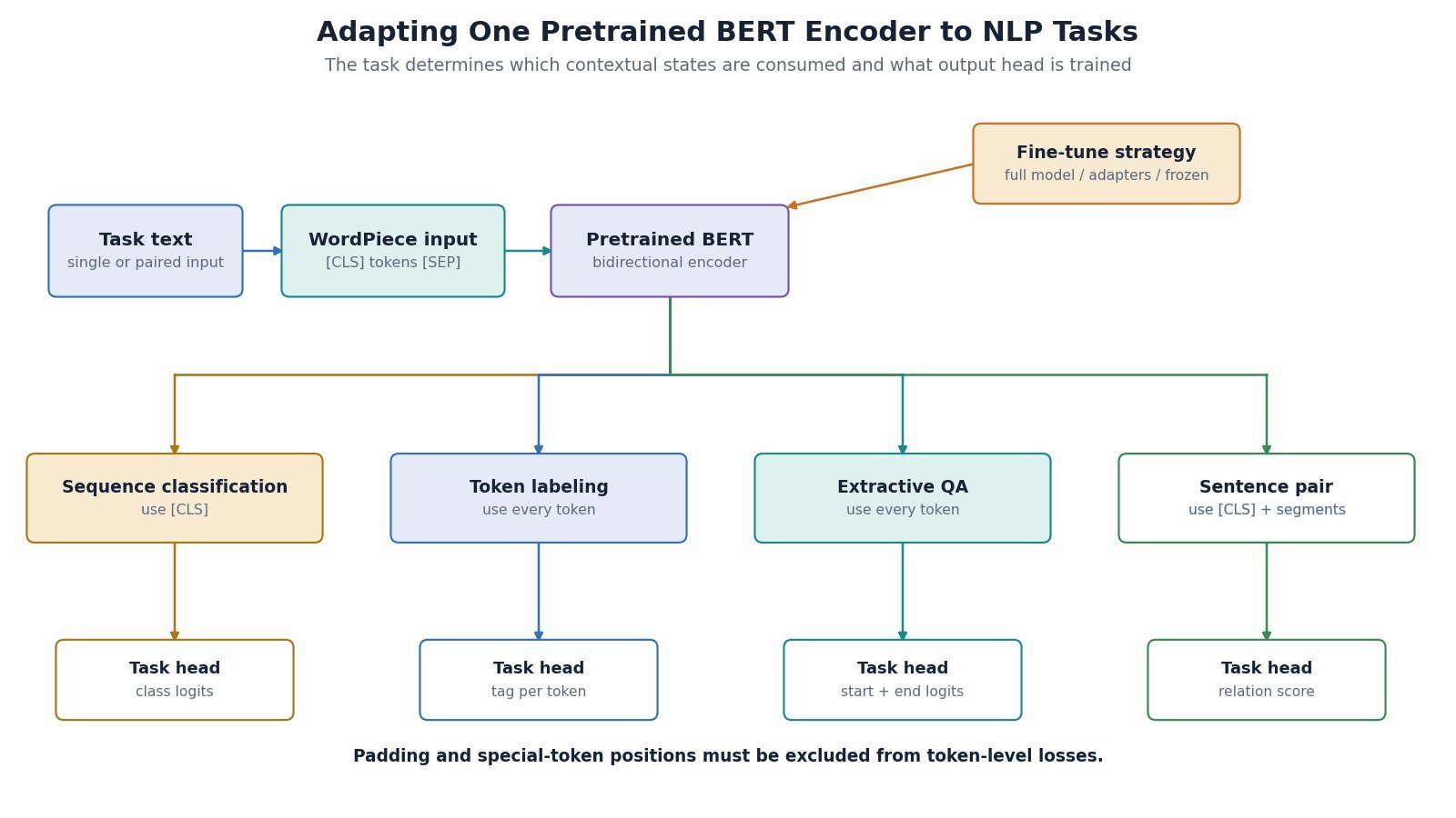

Figure 2: The same pretrained encoder can be adapted with small heads that consume either [CLS], every token state, or start/end span scores.
Login to view more content
July 20, 2026
DL0065 Group Normalization
What is Group Normalization?
Answer
Group Normalization normalizes each sample independently by dividing its channels into groups and computing a mean and variance over the channels and spatial positions within each group. The normalized activations then receive learned per-channel scale and shift parameters. Because its statistics do not depend on other examples, GroupNorm behaves consistently with very small or variable batch sizes and uses the same computation during training and inference. The group count must be compatible with the channel count, and its inductive bias can be less suitable than BatchNorm when large, stable batches provide useful batch statistics.
(1) Per-Sample Statistics: Each example has its own group means and variances, so no running batch averages are required.
(2) Channel Grouping: For $C$ channels and $G$ groups, each group normalizes $(C/G)\times H\times W$ values; channels within a group share statistics.
(3) Boundary Cases: $G=1$ normalizes all channels and spatial positions together, while $G=C$ gives one channel per group and resembles InstanceNorm.

Figure 1: A convolutional tensor is split into channel groups; each sample-group gets independent statistics before per-channel affine scaling.
Mathematical Formulation:
$\mu_{n,g}=\frac{1}{m}\sum_{i\in S_{n,g}}x_i$
$\sigma^2_{n,g}=\frac{1}{m}\sum_{i\in S_{n,g}}(x_i-\mu_{n,g})^2$
$y_{n,c,h,w}=\gamma_c\frac{x_{n,c,h,w}-\mu_{n,g(c)}}{\sqrt{\sigma^2_{n,g(c)}+\epsilon}}+\beta_c$
Where:
$n$ indexes samples, $g$ indexes channel groups, and $c,h,w$ index channel and spatial position.
$S_{n,g}$ is the set of activations in group $g$ of sample $n$ ; $i$ indexes elements in that set.
$m=(C/G)HW$ is the number of normalized values when $C$ channels are divided into $G$ groups over height $H$ and width $W$ .
$\mu_{n,g}$ and $\sigma^2_{n,g}$ are the group mean and variance; $x$ and $y$ are input and normalized output activations.
$g(c)$ maps channel $c$ to its group, $\gamma_c,\beta_c$ are learned per-channel scale and shift, and $\epsilon$ stabilizes division.

Figure 2: Normalization families differ mainly in which batch, channel, and spatial axes share statistics and whether inference needs running estimates.
Login to view more content
July 20, 2026
DL0064 CNNs Object Detection and Segmentation
What is the role of CNNs in object detection and segmentation?
Answer
In object detection and segmentation, a CNN commonly acts as a spatial feature extractor that converts pixels into a hierarchy of increasingly semantic feature maps. Detection heads use those features to classify objects and localize bounding boxes, while segmentation heads upsample and fuse spatial detail to predict per-pixel classes or instance-specific masks. Multiscale features are important because small objects need high-resolution maps and large objects benefit from deeper receptive fields. CNNs are therefore the backbone and often part of the head, but proposal logic, feature pyramids, decoders, and task losses complete the system; modern vision Transformers can also replace or complement the CNN backbone.
(1) Shared Backbone: Convolutions provide translation-equivariant local processing and reusable feature maps at several strides.
(2) Detection Role: One-stage or region-based heads turn features into class scores and box coordinates, often using multiscale pyramids.
(3) Segmentation Role: Dense decoders combine semantic context with fine spatial detail for semantic labels, instance masks, or panoptic outputs.

Figure 1: A shared convolutional feature hierarchy supports two different outputs: sparse boxes and classes versus dense semantic or instance masks.
Mathematical Formulation:
$F_l=\mathrm{CNN}_l(I)$
$(\hat b,\hat p)=H_{\mathrm{det}}(\{F_l\})$
$\hat M=H_{\mathrm{seg}}(\{F_l\})$
$\hat M\in\mathbb{R}^{H\times W\times K}$
Where:
$I$ is the input image and $F_l$ is the backbone feature map produced by stage $l$ .
$\{F_l\}$ is the multiscale feature set supplied to task heads.
$H_{\mathrm{det}}$ is the detection head, with $\hat b$ denoting predicted boxes and $\hat p$ predicted class probabilities.
$H_{\mathrm{seg}}$ is the segmentation head and $\hat M$ is its dense output mask or logit tensor.
$H$ and $W$ are output height and width, while $K$ is the number of semantic classes or mask channels.

Figure 2: Task-specific paths after the backbone show what each head must predict and how its output aligns with the input image.
Login to view more content
July 20, 2026
DL0063 Transformer Variable Length Sequences
How does the Transformer handle variable-length sequences?
Answer
A Transformer can process different sequence lengths because self-attention is defined over whatever number of tokens is supplied, up to the model’s context limit. For efficient batching, implementations usually pad sequences to a common length or group examples of similar lengths, then apply a padding mask so valid queries cannot attend to padded keys and values. Decoder-style models also add a causal mask that blocks future positions, while positional encodings identify token order within each sequence. Padded query outputs and losses must be ignored, and computation still scales with the padded batch length rather than only the number of valid tokens.
(1) Batch Construction: Sequences are dynamically padded to the longest item in a batch, bucketed by length, or packed by specialized kernels to reduce wasted work.
(2) Attention Masking: A key-padding mask removes padded keys and values from attention; causal models combine it with a triangular future mask.
(3) Length Boundary: Variable length does not mean unlimited length: positional support, memory, and the configured context window impose a maximum.

Figure 1: Unequal token sequences become a rectangular batch; masking separates valid context, padding, and future positions.
Mathematical Formulation:
$\mathrm{Attention}(Q,K,V)=\mathrm{softmax}\!\left(\frac{QK^\top}{\sqrt{d_k}}+M_{\mathrm{pad}}+M_{\mathrm{causal}}\right)V$
$M_{ij}\in\{0,-\infty\}$
Where:
$Q$ , $K$ , and $V$ are query, key, and value matrices, and $d_k$ is the key width used for score scaling.
$M_{\mathrm{pad}}$ assigns $-\infty$ to padded key positions so their softmax probabilities become zero.
$M_{\mathrm{causal}}$ assigns $-\infty$ when key index $j$ is later than query index $i$ ; encoder-only models normally omit this mask.
$M_{ij}$ denotes one combined mask entry and is either $0$ for an allowed connection or $-\infty$ for a blocked connection.
$B$ is batch size and $L_{max}$ is padded sequence length, giving a dense token tensor of shape $B\times L_{max}$ .

Figure 2: A practical variable-length pipeline: tokenize, bucket or pad, build masks, run attention, then ignore padded outputs or continue autoregressive generation.
Login to view more content
July 20, 2026
DL0061 Channel and Spatial Attention
Explain channel attention and spatial attention in CNNs. What information does each mechanism model?
Answer
Channel attention learns which feature channels are important, answering what semantic responses should be emphasized. It compresses spatial dimensions into channel descriptors, transforms them with a small gating network, and multiplies the resulting weights into the feature tensor. Spatial attention learns where informative regions occur by compressing or projecting the channel dimension and producing an $H\times W$ mask. Modules such as SE use channel attention, while CBAM applies channel attention followed by spatial attention to refine both feature type and location.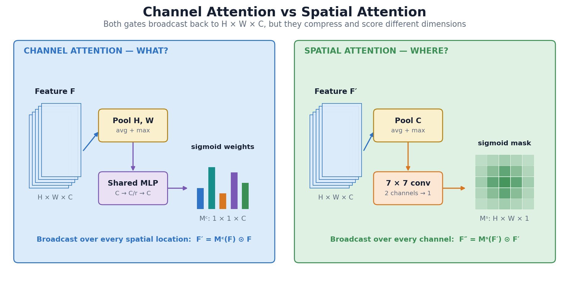
(1) Channel Gate: Global pooling summarizes each channel; an MLP or 1D convolution captures inter-channel dependence and outputs $C$ multiplicative weights.
(2) Spatial Gate: Average/max pooling or learned projection across channels produces spatial descriptors that a convolution maps to one $H\times W$ attention mask.
(3) Residual Placement: Attention usually modulates an existing feature tensor and is often inserted inside a residual block; sigmoid gates reweight rather than replace the underlying features.

Figure 1: Parallel tensor-shape explanation of what channel attention selects and where spatial attention focuses.
Mathematical Formulation:
$M_c(F)=\sigma\!\left(\mathrm{MLP}(\mathrm{AvgPool}_{hw}(F))+\mathrm{MLP}(\mathrm{MaxPool}_{hw}(F))\right)$
$M_s(F)=\sigma\!\left(f^{7\times7}([\mathrm{AvgPool}_{c}(F);\mathrm{MaxPool}_{c}(F)])\right)$
Where:
$F\in\mathbb{R}^{H\times W\times C}$ is the input feature map with height $H$ , width $W$ , and $C$ channels.
$M_c(F)\in\mathbb{R}^{1\times1\times C}$ is the channel mask; spatial average/max pooling and the shared $\mathrm{MLP}$ produce channel logits.
$M_s(F)\in\mathbb{R}^{H\times W\times1}$ is the spatial mask; channel pooling outputs are concatenated by $[\,;\,]$ and filtered by $f^{7\times7}$ .
$\sigma$ is the sigmoid function; $M_c$ broadcasts over $H,W$ , while $M_s$ broadcasts over $C$ .

Figure 2: CBAM data flow from input feature through channel gating, spatial gating, residual refinement, and output.
Login to view more content
July 20, 2026