
What is depthwise separable convolution, and where is it commonly used?
Answer
Depthwise separable convolution factorizes a standard convolution into a depthwise spatial operation and a pointwise channel-mixing operation. The depthwise stage applies one  filter per input channel, so it learns spatial patterns independently; the
  pointwise stage combines those channel responses into new output channels. This factorization can reduce multiply-accumulates and parameters by almost the kernel area when channel counts are large. It is common in MobileNet, Xception, EfficientNet-style mobile blocks, and edge models where latency, power, and model size matter.
(1) Depthwise Stage: With depth multiplier one,  independent filters produce spatially filtered maps and do not mix channels.
(2) Pointwise Stage: A convolution applies a learned  channel transformation independently at every spatial position.
(3) Real Hardware: Lower arithmetic cost does not guarantee proportional speedup because memory traffic, kernel launch overhead, vectorization, and accelerator support can dominate.
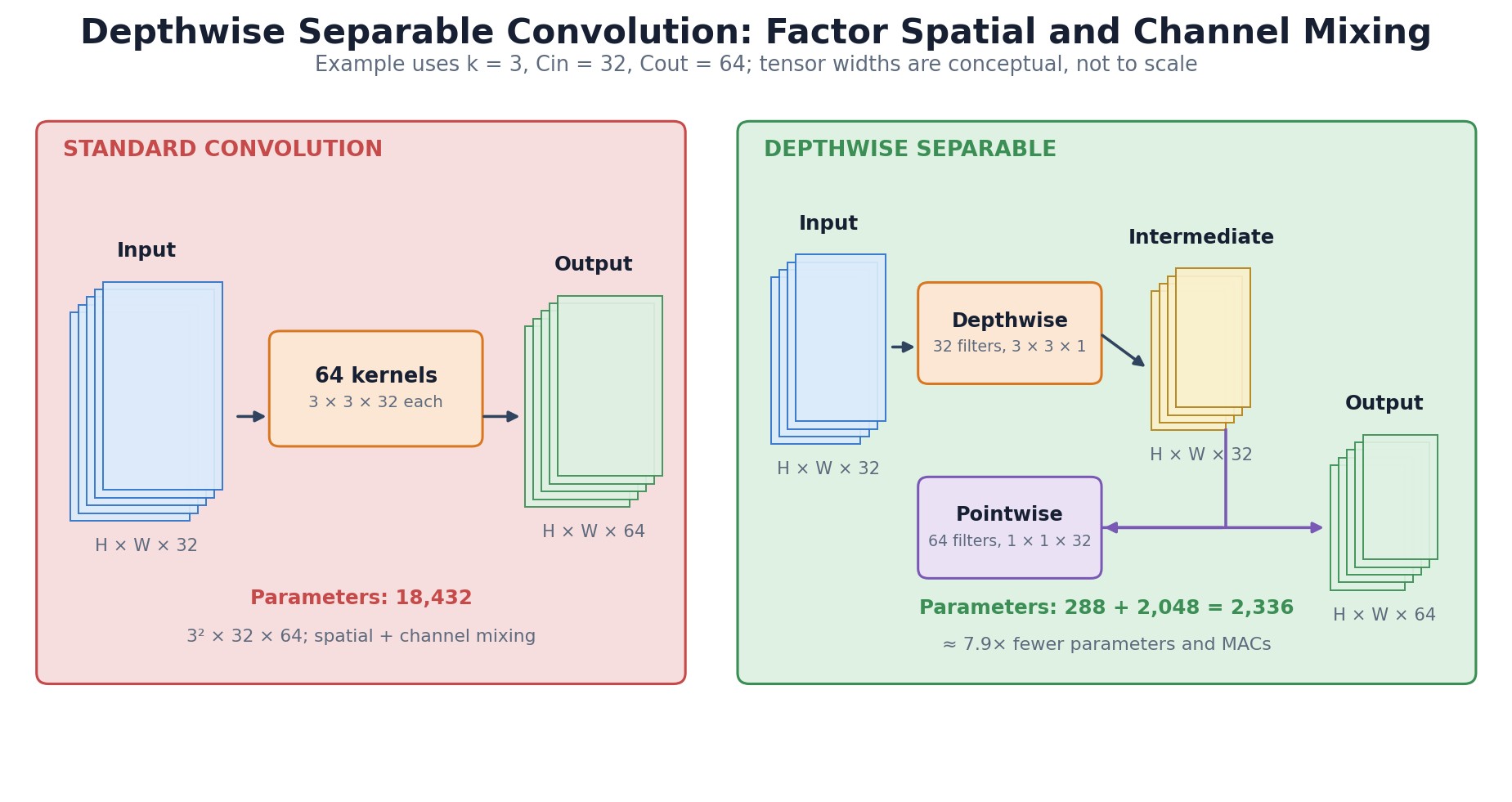
Figure 1: Tensor-level view of spatial filtering per channel followed by 1×1 channel mixing, with parameters and MACs.
Mathematical Formulation:


Where:
 and
and  count multiply-accumulates for standard and depthwise-separable convolution.
 and
and  are output height and width, and
  is the square spatial-kernel width.
 and
and  are input and output channel counts; the formula assumes depth multiplier
  .
.- For
 and large , the ratio approaches
  .
.
 and
and  count multiply-accumulates for standard and depthwise-separable convolution.
 and
and  are output height and width, and
  is the square spatial-kernel width.
 are input and output channel counts; the formula assumes depth multiplier
  .
. and large
  .
.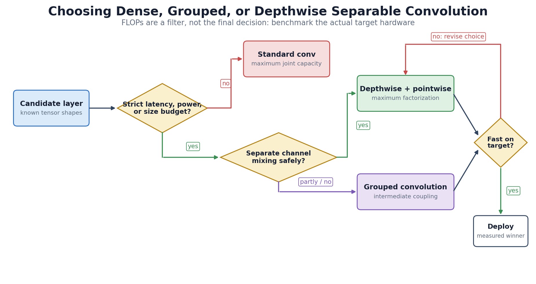
Figure 2: Architecture decision based on efficiency target, channel interaction, hardware kernels, and measured latency.
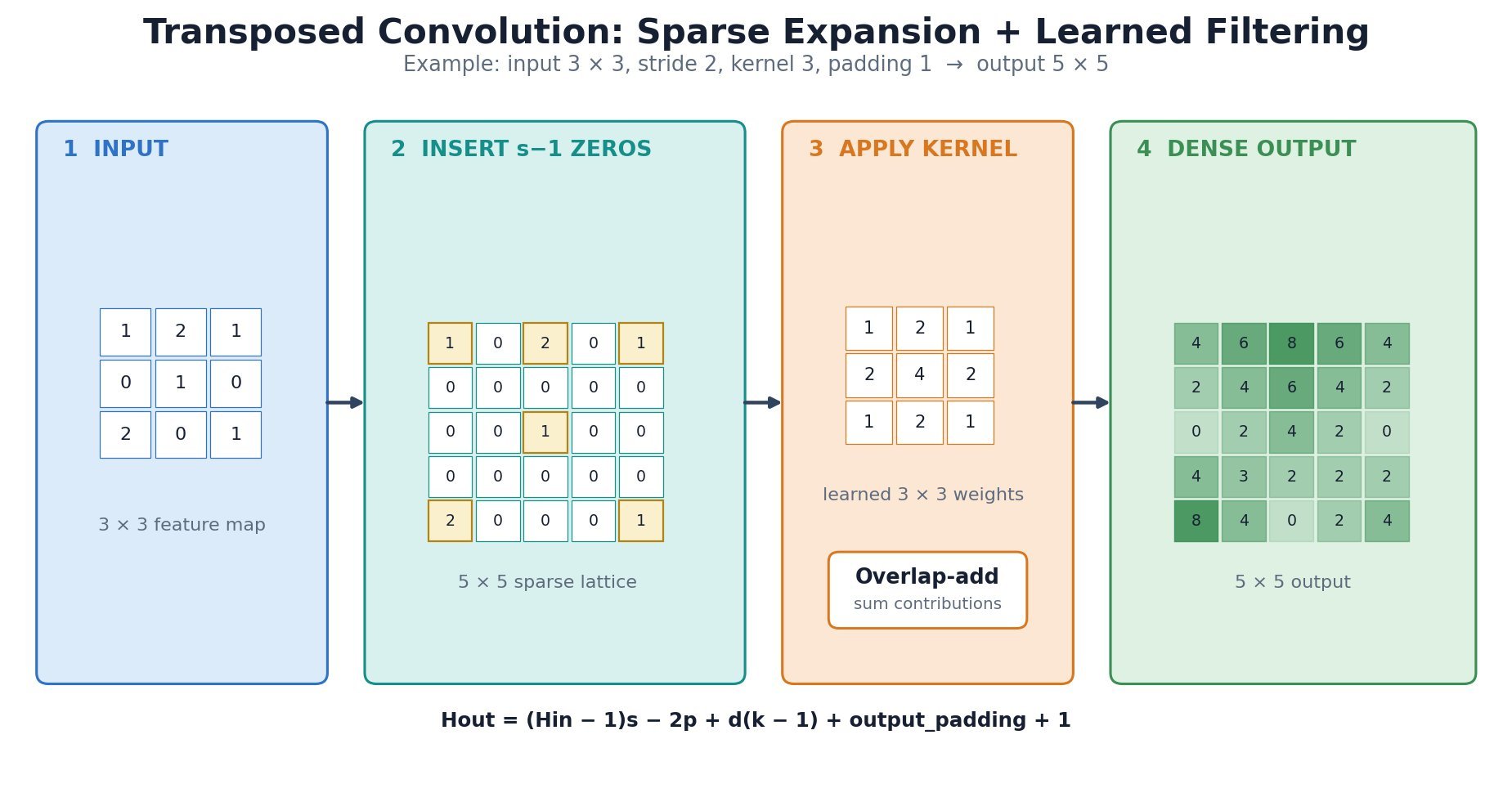

 and
and  are the input and output sizes along one spatial axis.
 is stride,
  is padding,
  is dilation, and
  is output padding used to choose among otherwise ambiguous valid output sizes; it does not append learned pixels.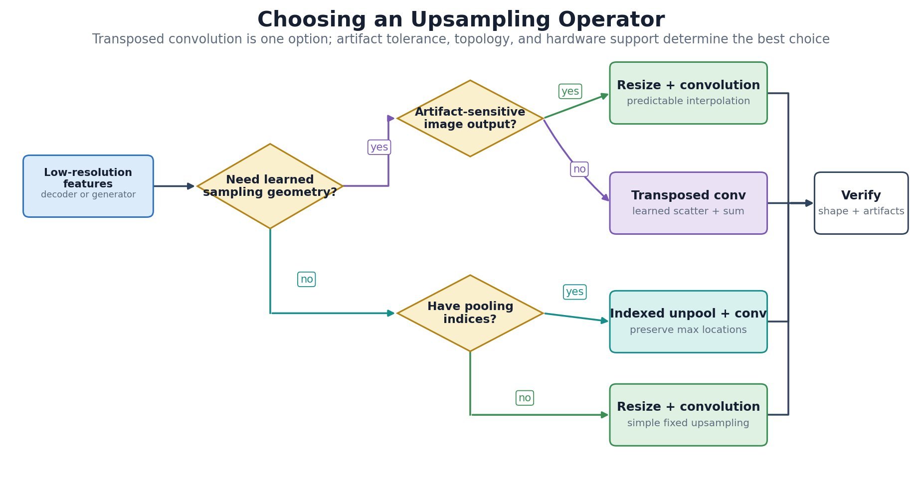
 maps combine localization detail with high-level context. Detection, instance segmentation, and keypoint heads can then select a pyramid level appropriate to each object or region scale.
 reduce spatial resolution while increasing receptive field and semantic abstraction.
 or
or  , while large objects use coarser levels such as
  or
or  .
.


 is the bottom-up backbone feature and
  is the fused pyramid output at level
  .
. aligns channel width,
  doubles spatial resolution, and
  smooths the merged feature.
 is the reference level, and
  are the region width and height.
 is the canonical reference scale and
  maps the continuous log-scale value to a discrete level.
 ; a 3D kernel adds
  and jointly traverses depth or time.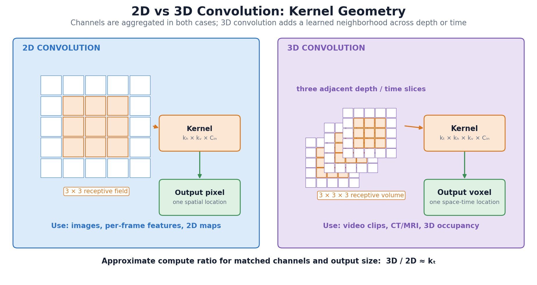

 and
and  are the input and output tensors, while
  is the learned 3D convolution kernel.
 indexes output channels and
  indexes input channels.
 index output depth/time, height, and width;
  range over the kernel support along those axes.
 are removed, leaving only spatial indices
  ; stride, padding, and dilation modify each active index mapping.
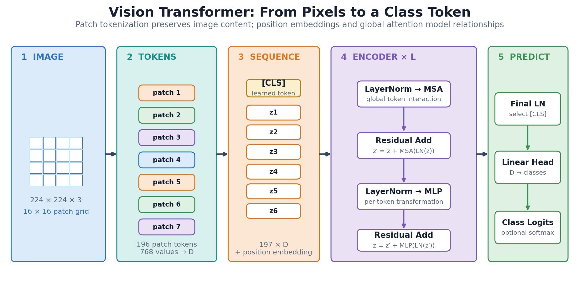
 is divided into
  non-overlapping
  patches; each flattened patch is projected to width
  .
.
![z_0=[x_{\mathrm{cls}};x_p^1E;x_p^2E;\ldots;x_p^NE]+E_{\mathrm{pos}}](https://s0.wp.com/latex.php?latex=z_0%3D%5Bx_%7B%5Cmathrm%7Bcls%7D%7D%3Bx_p%5E1E%3Bx_p%5E2E%3B%5Cldots%3Bx_p%5ENE%5D%2BE_%7B%5Cmathrm%7Bpos%7D%7D&bg=ffffff&fg=000&s=3&c=20201002)

 is the initial token sequence supplied to the Transformer encoder.
 is the learned class token, and
  is flattened image patch
  .
. projects each
  patch to width
  supplies positional embeddings.
 .
. ,
,  are query, key, and value matrices;
  is the per-head query/key width.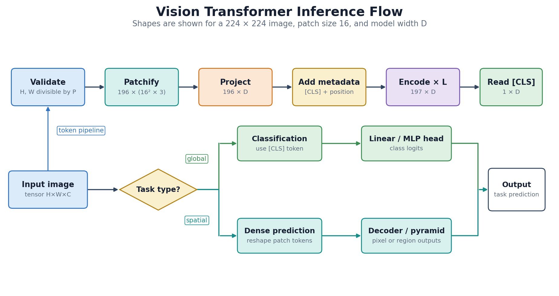
 to
to  where K is a small constant (typically 4). This makes it ideal for high-resolution feature maps in object detection where full attention is computationally prohibitive — for a 1024×1024 feature map (
 positions), standard attention requires ~1T operations per head while deformable attention needs only ~4M.
 positions, deformable attention samples only K reference points per query, typically K=4 or 8, reducing the key-value set from N to K.
 offsets from each reference point
  using a lightweight linear layer on query features, requiring only
  additional computation where C is channel dimension.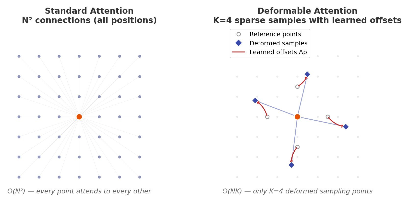
![y(p) = \sum_{m=1}^{M} W_m \left[ \sum_{k=1}^{K} A_{mk} \cdot W_m' x(p + p_k + \Delta p_{mk}) \right]](https://s0.wp.com/latex.php?latex=y%28p%29+%3D+%5Csum_%7Bm%3D1%7D%5E%7BM%7D+W_m+%5Cleft%5B+%5Csum_%7Bk%3D1%7D%5E%7BK%7D+A_%7Bmk%7D+%5Ccdot+W_m%27+x%28p+%2B+p_k+%2B+%5CDelta+p_%7Bmk%7D%29+%5Cright%5D&bg=ffffff&fg=000&s=3&c=20201002)
 is the reference position (query location on the feature map)
 is the number of attention heads
 is the number of sampled keys per head (typically 4)
 are fixed reference offsets (uniformly initialized)
 are learned deformable offsets (2D, predicted per head per key)
 is the attention weight (normalized, not from softmax over all positions)
 are projection matrices for each head
 , where
  . The attention weights
  are computed via a separate softmax over only K elements, not the full N positions. In Deformable DETR, multi-scale deformable attention extends this to sample across multiple feature map resolutions simultaneously, enabling the model to capture both small and large objects efficiently.
 is multiplied by a sigmoid gate
  where
where  is a head-specific projection.
![[0, 1]](https://s0.wp.com/latex.php?latex=%5B0%2C+1%5D&bg=ffffff&fg=000&s=2&c=20201002) , and empirical measurements show mean gate activation of ~0.116, meaning most heads are heavily suppressed — introducing beneficial sparsity without hard pruning.
, and empirical measurements show mean gate activation of ~0.116, meaning most heads are heavily suppressed — introducing beneficial sparsity without hard pruning.


 is the output of the
 ![g_i \in [0, 1]](https://s0.wp.com/latex.php?latex=+g_i+%5Cin+%5B0%2C+1%5D+&bg=ffffff&fg=000&s=2&c=20201002) is the head-specific gate score
is the head-specific gate score is a learned projection from query to scalar gate
 is the sigmoid function
 denotes element-wise multiplication
 is the standard output projection
 adds only
  parameters per head — a negligible overhead of ~0.1% of total model parameters — yet significantly improves long-context performance. On the RULER benchmark at 128K context length, gated attention improves needle-in-haystack retrieval accuracy from ~72% to ~94% compared to standard attention.
 composed with one at position
  depends only on the difference, the attention dot product between tokens automatically reflects their relative distance, with no learned parameters and good length generalization. RoPE is the default in GPT-NeoX, LLaMA, PaLM, Qwen, and most modern LLMs.
 , where
  the per-dimension frequency.
 only: absolute rotations yield relative-position attention.

 are one 2D pair of the query/key vector.


 is the
  controlling sparsity strength.
 is a neuron’s pre-activation input; ReLU’s hard zero is the simplest source of activation sparsity.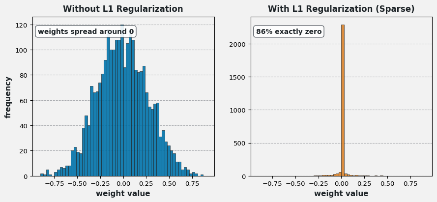
 , exposing inter-class similarity structure that hard labels hide.

 is the logit for class
  the temperature; higher
  yields a smoother distribution.
 balances hard-label CE against distillation; the
  factor rescales the KL term because softening shrinks its gradients by
  .
.
 only the winner class is visible; at higher