Category: Medium

  • DL0047 Focal Loss II

    Please compare focal loss and weighted cross-entropy.

    Answer

    Weighted cross-entropy (WCE) multiplies each class’s loss by a fixed weight \alpha_t: it corrects class frequency but treats every sample of a class identically. Focal loss (FL) adds a per-sample, difficulty-dependent factor (1 - p_t)^\gamma: it corrects prediction difficulty, automatically ignoring easy examples regardless of class. WCE is simple and robust; FL is stronger when an ocean of easy negatives overwhelms learning, but it can amplify noisy labels.

    (1) What Each Balances: WCE reweights by class prior; FL reweights by per-sample hardness (and can include \alpha_t too).
    (2) Gradient Behavior: WCE still lets millions of correctly-classified negatives contribute steady gradient; FL drives their contribution toward zero.
    (3) Robustness: WCE has one interpretable hyperparameter and is safe with noisy labels; FL’s focus on hard examples can overfit label noise and needs tuned \gamma, \alpha_t.

    Mathematical Formulation:
    \mathrm{WCE}(p_t) = -\alpha_t \log(p_t)
    \mathrm{FL}(p_t) = -\alpha_t (1 - p_t)^\gamma \log(p_t)

    Where:

    • p_t is the model’s predicted probability for the ground-truth class; \alpha_t is the fixed per-class weight.
    • \gamma \geq 0 is the focusing parameter, the entire difference between the two losses; at \gamma = 0 focal loss collapses to WCE.
    PropertyWeighted Cross-EntropyFocal Loss
    Handles class imbalanceYes: fixed class weightsYes: class weight + hardness factor
    Focuses on hard samplesNo: easy samples still dominateYes: easy samples fade to zero
    HyperparametersOne: \alpha_tTwo: \gamma and \alpha_t
    Main riskUnderwhelming at extreme imbalanceOverfits noisy / mislabeled hard examples

    Table 1: WCE vs focal loss: the same class weighting, but only focal loss adds per-sample difficulty weighting.

    Curves of cross-entropy, weighted cross-entropy at two alpha values, and focal loss at several gamma values versus true-class probability, showing WCE as a uniform vertical rescale while focal loss bends the curve down at high probability.

    Figure 1: WCE rescales the CE curve uniformly (same shape, different height); focal loss bends the shape, crushing the high-p_t (easy) region toward zero.

    Rule of Thumb: Moderate imbalance (up to ~10:1) → WCE is enough; extreme imbalance with floods of easy negatives (dense detection, 1000:1) → focal loss; noisy labels → prefer WCE.


    Login to view more content
  • DL0045 Dimension in FFN

    In Transformers, why does the feed-forward network expand the hidden dimension (e.g.,  d_{\text{model}} 4 d_{\text{model}} ) before reducing it back?

    Answer

    The FFN expands each token’s representation from d_{\text{model}} to 4 d_{\text{model}} to create a wide nonlinear workspace: in the higher-dimensional space the activation function can carve out far richer feature combinations than the residual stream’s width allows. It then projects back down so the result matches the residual stream for the skip connection and the next sub-layer. It is a bottleneck design that buys expressiveness where it is cheap while keeping the inter-layer interface narrow.

    (1) Extra Capacity: The wider hidden layer holds more features; the FFN is where most of a block’s parameters (8 d^2, about two-thirds) live.
    (2) Nonlinear Mixing: The activation (ReLU/GELU/SwiGLU) acts in the expanded space, letting the network represent sparse, high-order interactions that a d-wide layer cannot.
    (3) Projection Back: Returning to d_{\text{model}} keeps residual compatibility and a uniform interface across all layers.

    Mathematical Formulation:
    \mathrm{FFN}(x) = W_2\, \sigma(W_1 x + b_1) + b_2

    Where:

    • x \in \mathbb{R}^{d_{\text{model}}} is the per-token input from the residual stream.
    • W_1 \in \mathbb{R}^{4 d_{\text{model}} \times d_{\text{model}}} expands the dimension, \sigma is the nonlinearity, and W_2 \in \mathbb{R}^{d_{\text{model}} \times 4 d_{\text{model}}} projects back down.
    Feed-forward network flow: input of width d-model expands through linear W1 to 4 times d-model, passes an activation, then linear W2 reduces it back to d-model output.

    Figure 1: The FFN hourglass: expand d \to 4d, activate in the wide space, reduce 4d \to d to rejoin the residual stream.

    Empirical Note: The 4x factor dates to the original Transformer and was kept by BERT/GPT because it reliably improves loss; modern SwiGLU models (LLaMA) use ~2.7x with three matrices so the parameter count stays comparable.


    Login to view more content
  • DL0044 Multi-Query Attention

    What is Multi-Query Attention in transformer models?

    Answer

    Multi-Query Attention (MQA) is a variant of multi-head attention where all query heads share a single key and value projection instead of each head owning its own K/V. The KV cache therefore stores one K/V pair per token rather than one per head, shrinking cache memory and bandwidth by a factor of h, which directly speeds up autoregressive decoding, usually with only a minor quality cost.

    (1) Structure: Queries are still projected into h distinct heads, but all of them attend against one shared K and one shared V.
    (2) Cache Savings: The per-token KV cache drops from O(n \cdot h \cdot d_k) to O(n \cdot d_k), hx smaller.
    (3) Trade-off: Slightly less expressive than full MHA (one key/value “view” of the sequence), which GQA later interpolates by sharing K/V across small groups of heads.

    Mathematical Formulation:
    \mathrm{head}_i = \mathrm{softmax}\!\left(\frac{Q_i K_{\text{shared}}^{\top}}{\sqrt{d_k}}\right) V_{\text{shared}}
    \mathrm{Cache}_{\text{MQA}} = \frac{1}{h}\,\mathrm{Cache}_{\text{MHA}}

    Where:

    • Q_i is the query of head i \in \{1, \ldots, h\}; K_{\text{shared}}, V_{\text{shared}} are the single key/value projections used by all heads.
    • d_k is the head dimension and h the number of query heads.
    Side-by-side diagram of multi-head attention with separate query, key, and value boxes per head versus multi-query attention with many query heads converging on one shared key and value box.

    Figure 1: MHA gives every head its own K and V; MQA keeps multiple query heads but shares one K and one V across all of them.

    Why Decoding Gets Faster: Autoregressive inference is memory-bandwidth bound: every generated token must read the entire KV cache. An hx smaller cache means hx less data movement per step, which is why MQA (and its successor GQA, used in LLaMA-2/3) is standard in serving-oriented LLMs.


    Login to view more content
  • DL0042 Attention Computation

    Please break down the computational cost of attention.

    Answer

    Attention cost splits into a linear-in-n term from projections and a quadratic-in-n term from pairwise interactions. For sequence length n and model dimension d, the total is O(n d^2 + n^2 d): projections dominate for short sequences, while the n \times n score matrix dominates once n grows past d.

    (1) Q/K/V + Output Projections: Four d \times d GEMMs over n tokens: O(n d^2), linear in sequence length.
    (2) Score Matrix QK^\top and Value Mixing AV: Pairwise n \times n work: O(n^2 d), the quadratic bottleneck.
    (3) Softmax: Elementwise over n^2 entries: O(n^2), cheap FLOPs but the n \times n matrix drives memory traffic.

    Mathematical Formulation (one attention layer, h heads, d_k = d_v = d/h):
    \mathrm{Cost}_{\text{proj}} = O(n\, d^2)
    \mathrm{Cost}_{\text{scores}} = O(n^2\, d_k \cdot h) = O(n^2 d)
    \mathrm{Cost}_{\text{total}} = O\!\left(n^2 d + n\, d^2\right)

    Where:

    • n is the sequence length, d the model (hidden) dimension, and h the number of heads.
    • Q, K \in \mathbb{R}^{n \times d_k} form scores S = QK^\top \in \mathbb{R}^{n \times n}; attention weights A = \mathrm{softmax}(S / \sqrt{d_k}) mix values V \in \mathbb{R}^{n \times d_v} via O = AV.
    • Multi-head attention costs the same as single-head in big-O: per-head dimensions scale as d/h, so the h heads sum back to d.
    Log-log plot of attention and projection FLOPs versus sequence length at hidden dimension 512, with the quadratic attention term overtaking the linear projection term near n equals 512.

    Figure 1: Log-log cost curves at d = 512: projection O(n d^2) leads at short lengths, attention O(n^2 d) takes over near n \approx d and dominates at long context.

    Regimes: Short sequences (n \ll d): the n d^2 projection term dominates. Long sequences (n \gg d): the n^2 d interaction term dominates; the two balance around n \approx d.


    Login to view more content
  • DL0041 Hierarchical Attention

    Could you explain the concept of hierarchical attention in transformer architectures?

    Answer

    Hierarchical attention applies self-attention at multiple levels of granularity instead of one flat pass over all tokens: first local attention within segments (words inside a sentence, frames inside a shot), then global attention across the aggregated segment representations (sentences inside a document). This mirrors the natural structure of long inputs, cuts the quadratic cost dramatically, and yields interpretable focus at each level.

    (1) Local Level (Fine-Grained): Each segment runs its own self-attention over its tokens, producing one segment embedding; cost grows with segment length, not document length.
    (2) Global Level (Coarse-Grained): The segment embeddings attend over each other, producing a document-level representation.
    (3) Efficiency Gain: A document of n tokens split into s segments of m tokens costs O(s m^2 + s^2) in attention entries instead of O(n^2), a large saving when m \ll n.

    Two-level hierarchy diagram: word tokens attend inside sentence segments, sentence embeddings then attend globally to form a document embedding.

    Figure 1: Two attention levels: local attention inside each segment, then global attention over segment embeddings to form the document representation.

    Mathematical Formulation (cost for n = s × m tokens):
    \text{Flat:}\quad \mathrm{Cost} \propto n^2
    \text{Hierarchical:}\quad \mathrm{Cost} \propto \underbrace{s\, m^2}_{\text{local}} + \underbrace{s^2}_{\text{global}} \ll n^2

    Where:

    • n is the total token count, split into s segments of m tokens each (n = s \cdot m).
    • The local term runs s independent m \times m attentions; the global term runs one s \times s attention over segment embeddings.

    Example (Document Classification): With n = 4096 tokens as s = 64 sentences of m = 64 words, flat attention scores 16.8\text{M} pairs, while hierarchical attention scores only 64 \cdot 64^2 + 64^2 \approx 0.27\text{M}, roughly 60x fewer pairs.


    Login to view more content
  • DL0037 Transformer Architecture III

    Why do Transformers use a dot product, rather than addition, to compute attention scores?

    Answer

    The dot product is a natural similarity measure: q \cdot k is large exactly when query and key point in the same direction, so it directly expresses “how relevant is this key to my query”. It is also a single fused matrix multiplication (QK^\top scores all pairs at once), which is far faster on modern hardware than additive attention’s per-pair MLP. Scaling by 1/\sqrt{d_k} keeps it numerically stable in high dimensions.

    (1) Geometric Meaning: q \cdot k = \|q\|\,\|k\|\cos\theta: aligned vectors score high, orthogonal vectors score zero, opposed vectors score negative.
    (2) Hardware Efficiency: All scores materialize as one GEMM QK^\top; additive attention needs an MLP evaluated for every (query, key) pair.
    (3) Probabilistic Readout: Softmax over dot-product scores yields interpretable attention weights: a distribution over which keys matter.

    2D vector diagram showing three vectors from the origin with a positive dot product between two aligned vectors and a negative dot product between two opposed vectors.

    Figure 1: Dot product as similarity: aligned vectors score positive, opposed vectors score negative; softmax turns scores into attention weights.

    Mathematical Formulation:
    \alpha_i = \frac{e^{q \cdot k_i / \sqrt{d_k}}}{\sum_{j=1}^{n} e^{q \cdot k_j / \sqrt{d_k}}}

    Where:

    • \alpha_i is the attention weight the query assigns to key k_i; weights sum to 1 over the n keys.
    • q \cdot k_i is the dot-product similarity; \sqrt{d_k} scaling prevents softmax saturation for large key dimension d_k.

    Why Not Addition: Adding features component-wise, q + k, says nothing about alignment; two very different pairs can sum to the same vector. To become a usable score, the sum must pass through an extra learnable MLP (v^\top \tanh(W_q q + W_k k)), which is slower per pair and still lacks the dot product’s direct geometric interpretation.

    Comparison flowchart of dot-product attention scoring all pairs in one matrix multiply versus additive attention pushing each query-key pair through a small neural network scorer.

    Figure 2: Dot-product scoring = one batched GEMM; additive scoring = a per-pair MLP, richer but much slower at scale.

    The One Caveat: For large d_k, raw dot products grow in variance proportional to d_k, pushing softmax into saturated, gradient-poor regions, which is why the Transformer uses the scaled dot product rather than the plain one.


    Login to view more content
  • DL0029 Dilated Attention

    Could you explain the concept of dilated attention in transformer architectures?

    Answer

    Dilated attention sparsifies self-attention by letting each query attend only to every d-th key position (a strided subset of the sequence) instead of all keys or a contiguous window. Borrowed from dilated convolutions in CNNs, the dilation rate d controls the stride: attention keeps a long global reach (the sampled keys span the whole sequence) while computing only about 1/d of the score matrix. The trade-off is granularity: nearby fine detail is skipped within each head.

    (1) Strided Sampling: Query i attends to keys j where (j - i) is a multiple of d; d = 1 recovers full attention.
    (2) Global but Sparse: Unlike sliding windows, coverage spans the entire sequence: long-range links survive, sampled coarsely.
    (3) Cost Reduction: Each row computes roughly n/d scores, so compute and memory drop from O(n^2) toward O(n^2 / d).

    A 16x16 attention matrix where each query attends only to every third key position forming a regular striped dilated pattern with dilation rate three.

    Figure 1: Dilation d = 3: each query attends every 3rd key: full-span coverage with a third of the computations.

    Mathematical Formulation:
    \mathrm{Attention}_{dilated}(Q, K, V) = \mathrm{softmax}\left(\frac{Q K_d^{\top}}{\sqrt{d_k}}\right) V_d
    K_d, V_d = \text{rows of } K, V \text{ at strided (dilated) positions}

    Where:

    • d is the dilation rate, the stride between attended key positions.
    • K_d, V_d are the dilated subsets of keys and values (about n/d rows per query).
    • d_k is the key dimension, used for the usual softmax scaling.

    Coverage Through Stacking: Layers with increasing dilation rates (e.g., 1, 2, 4, 8) progressively widen and interleave coverage, so deeper layers see the full sequence even though each layer is sparse: the same trick as WaveNet’s exponentially dilated convolutions.

    Propagation of a single active position through two iterations of dilation-2 attention showing a regular grid of covered cells with gaps that never get attended.

    Figure 2: Gridding artifacts: repeating one fixed dilation leaves some positions permanently unattended. Mixing dilation rates closes the gaps.


    Login to view more content
  • DL0028 Sliding Window Attention

    Explain the sliding window attention mechanism in transformer architectures.

    Answer

    Sliding window attention restricts each token’s attention to a fixed-size local neighborhood instead of the whole sequence: token i attends only to tokens within roughly \pm w/2 positions of itself. This turns the dense n \times n attention matrix into a sparse band around the diagonal, cutting cost from O(n^2) to O(n \cdot w) and making Transformers practical for very long documents, at the price of losing direct long-range links within a single layer.

    (1) Local Window: Each token sees itself plus its w nearest neighbors; everything else is masked out before the softmax.
    (2) Linear Scaling in n: Cost per token is constant (w keys), so total compute and memory grow linearly with sequence length.
    (3) Trade-off: Excellent for local patterns, but global context must be recovered by stacking layers, adding global tokens, or mixing with dilated windows.

    Two attention matrices: a fully dense global attention matrix versus a sliding window matrix with attention confined to a band of width five around the diagonal.

    Figure 1: Global attention fills the whole n \times n matrix; the sliding window keeps only a diagonal band of width w.

    Mathematical Formulation:
    A_{ij} = \frac{q_i \cdot k_j}{\sqrt{d_k}} \quad \text{only if } |i - j| \leq \tfrac{w}{2}, \text{ else masked}
    \text{Cost: } O(n^2) \;\rightarrow\; O(n \cdot w), \quad w \ll n

    Where:

    • w is the window size (e.g., 512 in Longformer); tokens outside the window get -\infty scores before softmax.
    • n is the sequence length; with w fixed, memory and compute scale linearly in n.

    How Global Context Survives: Stacking L layers grows the effective receptive field to about L \cdot w tokens, similar to CNNs; Longformer additionally designates a few global tokens (e.g., [CLS], question tokens) that attend to and are attended by everything.
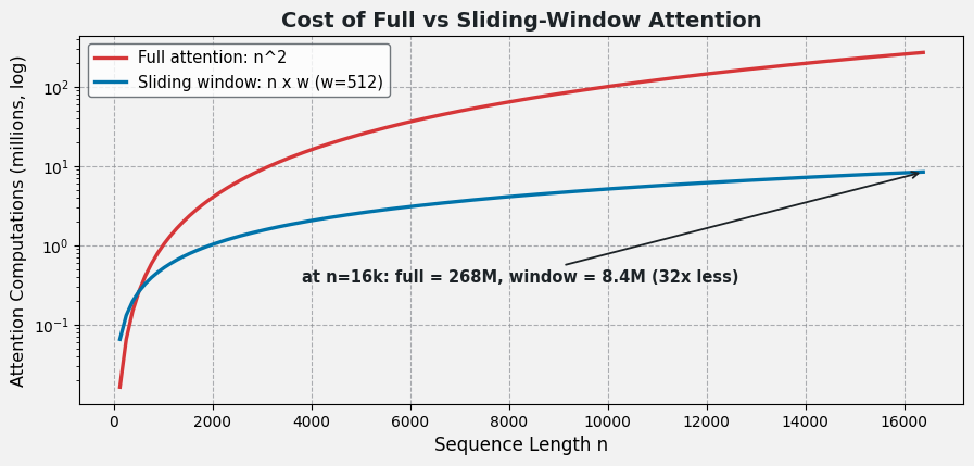
    Log-scale plot comparing n-squared full attention cost against n-times-w sliding window cost, with an annotation showing 32 times fewer computations at sequence length 16 thousand.

    Figure 2: At n = 16{,}384, full attention needs ~268M score computations versus ~8.4M for a 512-wide window, a 32x saving that grows with n.

    Used In: Longformer, BigBird (window + global + random blocks), and many long-document and code models where full O(n^2) attention is infeasible.


    Login to view more content
  • DL0024 Fixed-size Input in CNN

    What is the “dilemma of fixed-size input” for CNNs? How is it typically resolved?

    Answer

    The dilemma of fixed-size input is the constraint that classic CNN classifiers (VGG, early ResNets) only accept images of one predetermined resolution: the fully connected head has a weight matrix whose input dimension equals the flattened feature-map size, and that size is only constant if every input image has the same H \times W. Real-world images arrive in arbitrary sizes, so they must be resized or cropped first, distorting aspect ratios, discarding small objects, or cutting content away.

    (1) The FC Head Is the Bottleneck: Convolutions themselves handle any spatial size; only the flatten + FC stage pins the input dimensions.
    (2) Preprocessing Costs Information: Resizing squishes content and can erase small objects; cropping keeps resolution but discards everything outside the window.
    (3) Structural Fixes Exist: Replace or decouple the FC head (GAP, fully convolutional designs, or adaptive pooling) and the network accepts variable sizes natively.

    Three panels showing an original scene with one large and several small objects, a heavily downsampled version where the small objects disappear, and a center crop where objects near the edges are cut away.

    Figure 1: Both standard fixes hurt: downsampling erases small objects; cropping amputates anything near the border.

    Mathematical Formulation (Why the FC Head Fixes the Size):
    z = W \cdot \mathrm{vec}(X) + b, \quad X \in \mathbb{R}^{H \times W \times C}
    \mathrm{GAP}(X)_c = \frac{1}{HW} \sum_{h=1}^{H} \sum_{w=1}^{W} X_{hwc}

    Where:

    • X is the final feature volume; \mathrm{vec}(X) flattens it to HWC values, so W exists only for one specific H \times W.
    • \mathrm{GAP}(X)_c averages channel c over all spatial positions, yielding a C-dimensional vector for any input size.

    Common Solutions: (1) Global Average Pooling: replace the flatten with a per-channel average, so the classifier sees exactly C values regardless of resolution; (2) Fully Convolutional Networks: remove FC layers entirely and let the output scale with the input (standard for segmentation); (3) Adaptive Pooling: pool to a fixed k \times k grid no matter the input size (e.g., nn.AdaptiveAvgPool2d in PyTorch).

    Diagram of a variable-size input feeding three solution paths, global average pooling, fully convolutional network, and adaptive pooling, all converging to a fixed classifier head that accepts any input size.

    Figure 2: Three structural escapes (GAP, FCN, and adaptive pooling) all remove the fixed-size constraint at its source: the FC head.


    Login to view more content
  • DL0023 Dilated Convolution

    What are dilated convolutions? When would you use them?

    Answer

    Dilated convolutions (also called atrous convolutions) insert gaps between the elements of a convolutional kernel: with dilation rate d, the kernel samples every d-th input position instead of adjacent ones. This expands the receptive field without adding parameters and without reducing spatial resolution, a combination that pooling cannot offer. A dilation rate of 1 is just a standard convolution.

    (1) Larger Receptive Field, Same Weights: A 3×3 kernel with dilation 2 covers a 5×5 area but still has only 9 weights.
    (2) Resolution Preserved: Unlike pooling, dilation grows the receptive field while keeping the output the same size as a standard convolution, which is critical for dense prediction.
    (3) Multi-Scale Context: Stacking or mixing dilation rates lets one network aggregate both fine local detail and broad context.

    One-dimensional comparison of a standard kernel-3 convolution sampling three consecutive inputs versus a dilation-3 convolution sampling positions 0, 3, and 6 for a receptive field of seven with the same three weights.

    Figure 1: Same 3 weights, wider view: dilation 3 spreads the taps across a receptive field of 7 instead of 3.

    Mathematical Formulation:
    y_{ij} = \sum_{a=1}^{k}\sum_{b=1}^{k} w_{ab}\; x_{i + d \cdot a,\; j + d \cdot b}
    k_{eff} = k + (k - 1)(d - 1)

    Where:

    • d is the dilation rate, the spacing between tapped positions (d = 1 is standard convolution).
    • k is the nominal kernel size; k_{eff} is the effective span of the dilated kernel (3×3 with d = 2 behaves like 5×5 with holes).
    • w_{ab} are the kernel weights; the parameter count is independent of d.

    In Two Dimensions: The same idea applies to images: the kernel’s taps spread over a checkerboard-like stencil, expanding the covered span from 3×3 to 5×5 at dilation 2 while the channel count and output resolution stay unchanged.

    Two ten-by-ten grids comparing a dense 3x3 standard convolution stencil against a sparse 3x3 dilation-2 stencil that spans a 5x5 region marked by a red dashed receptive-field box.

    Figure 2: Dilation 2 turns a 3×3 stencil into a 5×5 receptive field (red dashed box), still only 9 multiply-accumulates.

    When to Use Them: Any task needing large context at full resolution: semantic segmentation (DeepLab), audio generation (WaveNet models long-range temporal structure with exponentially growing dilation), and dense tasks like super-resolution or depth estimation.

    Progression of a single input point through three stacked dilation-2 layers showing the response spreading into a checkerboard pattern with gaps between covered cells.

    Figure 3: Gridding artifacts: stacking the same dilation leaves a checkerboard of unattended cells. Mitigate with hybrid dilation rates (e.g., 1, 2, 5) that overlap coverage.


    Login to view more content