Tag: Transformer

  • DL0036 Transformer Architecture II

    What are the main differences between the encoder and decoder in a Transformer?

    Answer

    The encoder builds rich bidirectional representations of the source sequence: every token attends to every other token. The decoder is built for generation: its self-attention is causally masked so each position only sees the past, and it inserts an extra cross-attention sub-layer that reads the encoder’s output. Same building blocks, different wiring for two different jobs: understanding vs generating.

    (1) Self-Attention Masking: Encoder self-attention is unmasked (full bidirectional context); decoder self-attention is masked so position t attends only to \leq t.
    (2) Cross-Attention: Absent in the encoder; present in every decoder layer: queries from the decoder state, keys/values from the encoder output.
    (3) Inputs & Role: Encoder consumes the source sequence once; decoder consumes the shifted-right target (teacher forcing) and produces next-token distributions.

    Side-by-side encoder and decoder stacks separated by a dashed line, with the encoder's two sub-layers versus the decoder's three sub-layers and a cross-attention arrow bridging encoder output into the decoder.

    Figure 1: Two stacks, three differences: the decoder adds a causal mask on self-attention and a cross-attention bridge to the encoder output.

    Mathematical Formulation (decoder self-attention mask):
    \mathrm{Attn}(Q, K, V, M) = \mathrm{softmax}\left(\frac{QK^\top}{\sqrt{d_k}} + M\right)V
    M_{ij} = 0 \;\text{if}\; j \leq i,\quad -\infty \;\text{if}\; j > i

    Where:

    • M is the causal mask: -\infty above the diagonal zeroes out future positions after softmax; the encoder simply omits M.
    • i, j index query and key positions; j \leq i means “past or present only”.
    AspectEncoderDecoder
    Self-attentionUnmasked: all positionsMasked: past positions only (causal)
    Cross-attentionNot presentPresent: attends to encoder outputs
    Positional encodingAdded to source embeddingsAdded to target embeddings (shifted right)
    InputSource sequenceShifted target + encoder outputs
    FunctionEncode source into contextual representationsGenerate target autoregressively with source context

    Table 1: Encoder vs decoder at a glance. The decoder is a superset: same sub-layers plus masking and the cross-attention bridge.
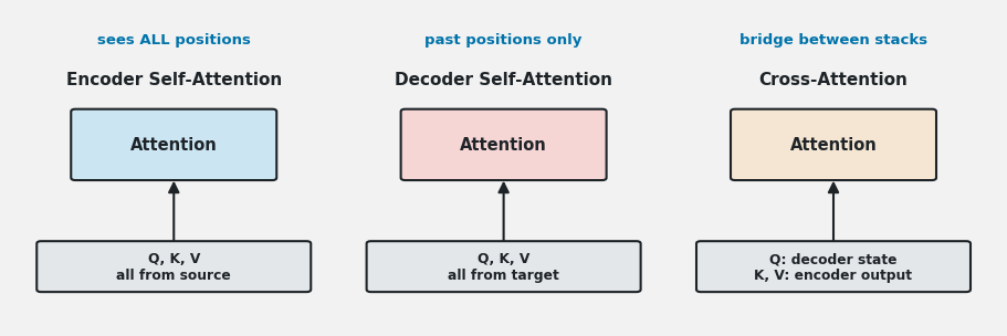
    Three mini diagrams showing query key value sources for encoder self-attention, masked decoder self-attention, and cross-attention with queries from the decoder and keys and values from the encoder output.

    Figure 2: Q/K/V sources for the three attention types: only cross-attention mixes sequences: Q from the decoder, K/V from the encoder.

    Why “Shifted Right”: During training the decoder receives the target sequence shifted one position right (prefixed with a start token), so the prediction at position t is supervised against token t while the input only ever reveals tokens before it. This is teacher forcing, and it keeps training fully parallel despite autoregressive inference.


    Login to view more content
  • DL0035 Transformer Architecture

    Describe the original Transformer encoder–decoder architecture.

    Answer

    The original Transformer (Vaswani et al., 2017) is a sequence-to-sequence encoder–decoder built entirely from attention: no recurrence, no convolution. The encoder (6 stacked layers) reads the full source sequence and builds a contextual representation per token; the decoder (6 stacked layers) generates the target sequence one token at a time, attending both to its own past outputs and to the encoder’s representations.

    (1) Encoder Layer: Multi-head self-attention (unmasked, so every token sees all positions) followed by a position-wise FFN, each wrapped in residual + LayerNorm.
    (2) Decoder Layer: Masked multi-head self-attention (no peeking at future tokens), then cross-attention to the encoder output, then an FFN, again with residual + LayerNorm throughout.
    (3) Input/Output: Token embeddings plus positional encodings feed both stacks; the decoder’s top passes through a linear + softmax head for next-token probabilities.

    Compact diagram of the original Transformer showing the encoder stack on the left and decoder stack on the right, with cross-attention flowing from encoder output into every decoder layer and a linear softmax head on top.

    Figure 1: The original architecture: 6 encoder layers build source representations; 6 decoder layers generate autoregressively, bridged by cross-attention.

    Mathematical Formulation (one sub-layer):
    z = \mathrm{LayerNorm}\big(x + \mathrm{Sublayer}(x)\big)

    Where:

    • x is the sub-layer input (n \times d_{model} matrix of token vectors, d_{model} = 512).
    • \mathrm{Sublayer} is multi-head self-attention, cross-attention, or the FFN; the residual add + LayerNorm pattern wraps every sub-layer in both stacks.
    Flowchart inside one encoder layer showing input splitting into multi-head self-attention then add-and-norm then feed-forward then add-and-norm, with residual bypass arrows around each sub-layer.

    Figure 2: Inside one encoder layer: two sub-layers (MHA, FFN), each followed by add & norm; the decoder adds a masked self-attention and cross-attention stage.

    Why the Design Works: Self-attention gives every token direct access to every other token (no information bottleneck through a fixed hidden state), residual connections + LayerNorm keep 12-deep training stable, and the masked decoder preserves causality so training can run in parallel via teacher forcing while inference stays autoregressive.


    Login to view more content
  • DL0034 Layer Norm

    What is layer normalization, and why is it used in Transformers?

    Answer

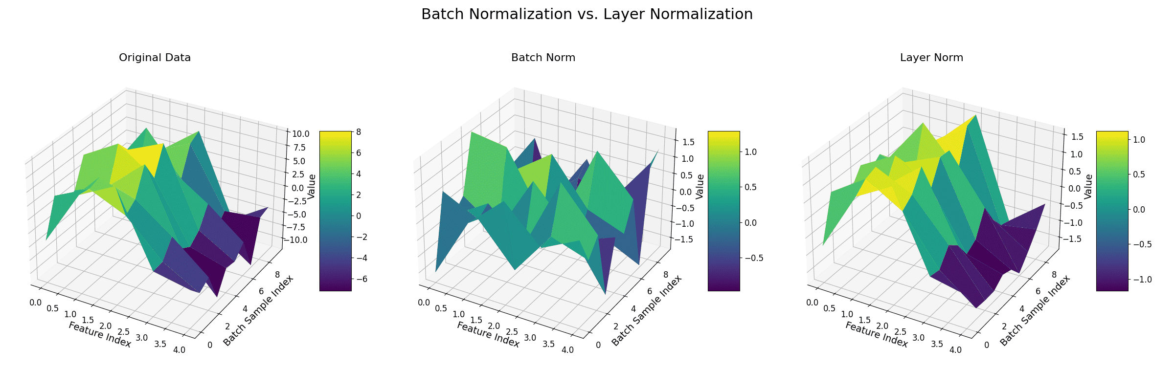
    Layer Normalization (LN) standardizes the features of each individual sample: for one token’s embedding vector, it computes the mean and variance across the feature dimension only, rescales to zero mean and unit variance, then applies a learnable scale and shift. Unlike BatchNorm, it never looks across the batch, which is exactly why Transformers, with variable-length sequences and small or on-the-fly batches, rely on it in every block.

    (1) Normalization Within a Sample: Mean and variance come from the d_{model} features of a single token: one set of statistics per token, not per batch.
    (2) Batch-Size Independence: Behavior is identical at train and test time and for any batch size: no running statistics, no mismatch.
    (3) Stabilizes Training: Keeps activations in a consistent range, preventing exploding/vanishing gradients and enabling deep stacks to converge faster.

    3D illustration of Layer Normalization: each sample (row) is normalized across its own feature dimensions, independent of the other samples in the batch.

    Figure 1: Layer Normalization standardizes each sample (row) across its own feature dimensions; statistics never cross sample boundaries, so batch size is irrelevant.

    Mathematical Formulation:
    \hat{x}_i = \frac{x_i - \mu}{\sqrt{\sigma^2 + \epsilon}} \cdot \gamma + \beta
    \mu = \frac{1}{d}\sum_{i=1}^{d} x_i
    \sigma^2 = \frac{1}{d}\sum_{i=1}^{d}(x_i - \mu)^2

    Where:

    • x_i is one feature of a single token’s d-dimensional vector; statistics are computed over i = 1..d for that token alone.
    • \epsilon is a small constant for numerical stability; \gamma, \beta are learnable per-feature scale and shift that restore representational freedom.

    Why Not BatchNorm: BatchNorm’s statistics mix information across samples, degrade with small or variable-size batches, behave differently at train vs inference, and pad tokens corrupt the per-feature means of variable-length sequences: all fatal for typical Transformer workloads.

    Two mini flowcharts of a Transformer sub-layer contrasting Post-LN where normalization follows the residual addition with Pre-LN where normalization precedes the sub-layer and the residual path stays clean.

    Figure 2: Placement variants: original Post-LN (after the residual add) vs modern Pre-LN (inside the residual branch), which keeps a clean gradient highway.

    Where It Sits: Every attention and FFN sub-layer is wrapped as \mathrm{LN}(x + \mathrm{Sublayer}(x)) (Post-LN) in the original paper; most modern LLMs use Pre-LN, normalizing the sub-layer input instead, which trains stably even without learning-rate warmup.


    Login to view more content
  • DL0033 Transformer Computation

    In a Transformer architecture, which components are the primary contributors to computational cost, and why?

    Answer

    It depends on sequence length. For short sequences, the feed-forward network (FFN) usually dominates: its two wide GEMMs cost O(n d^2) while attention’s quadratic term is still small. For long sequences, multi-head attention takes over: forming the n \times n score matrix costs O(n^2 d) and grows much faster than anything else in the block.

    (1) Multi-Head Attention: Q/K/V projections cost O(nd^2), but the score matrix QK^\top and its product with V cost O(n^2 d), the quadratic term that explodes on long sequences.
    (2) Feed-Forward Network: Two dense layers with expansion factor 4 cost O(nd^2), dominant when n is small but d is large.
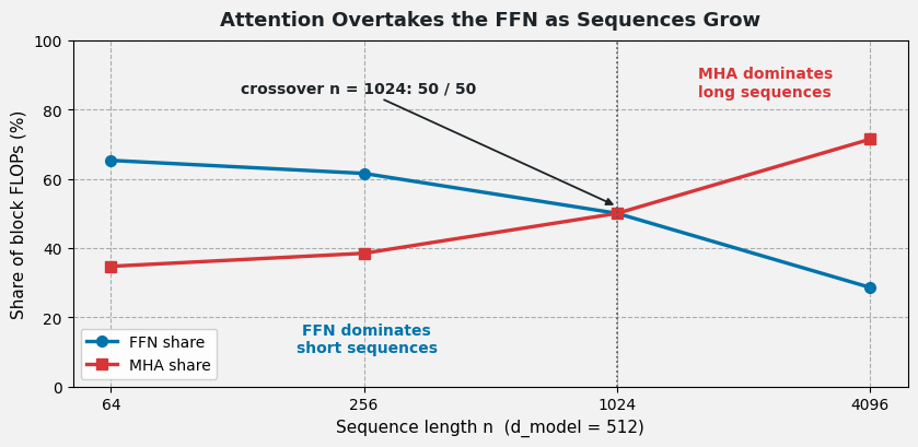
    (3) Crossover Point: Attention overtakes the FFN roughly when n \approx 2d; near n = 1024 for the classic d_{model} = 512 design.

    Line chart of MHA and FFN share of total FLOPs versus sequence length on a log scale, crossing at sequence length 1024 where each takes fifty percent.

    Figure 1: FLOP share vs sequence length (d = 512): FFN dominates below n \approx 1024; past the crossover, attention’s quadratic cost becomes the bottleneck.

    Mathematical Formulation (per block):
    \text{Cost}_{\text{attn}} = \underbrace{4nd^2}_{\text{QKVO projections}} + \underbrace{2n^2 d}_{QK^\top \text{ and } AV}
    \text{Cost}_{\text{FFN}} = 2 \cdot n \cdot d \cdot 4d = 8nd^2

    Where:

    • n is the sequence length and d = d_{model}; constants count multiply–adds per GEMM.
    • The 2n^2 d term comes from multiplying (n \times d) \cdot (d \times n) to form scores, and again to mix values.
    • Softmax itself is cheap elementwise work but also scales with n^2 entries.
    Sequence Length nMHA Share (%)FFN Share (%)Dominant Component
    6434.6965.31FFN
    25638.4661.54FFN
    102450.0050.00Tie
    409671.4328.57MHA

    Table 1: FLOP breakdown at d = 512: the tie at n = 1024 marks where quadratic attention catches up with the linear-in-n FFN.

    Flowchart of one Transformer block annotating each operation with its FLOP complexity: projections linear in n, score matrix quadratic in n, FFN linear in n but quadratic in d.

    Figure 2: Where the FLOPs live inside one block: only the QK^\top and AV pair grows quadratically with sequence length.

    Practical Caveat: The FFN’s dominance at short n assumes the standard 4x expansion; shrink the expansion to 1x and the Q/K/V projections become the largest term, while efficient attention variants (sliding-window, linear attention) specifically attack the n^2 term for long contexts.


    Login to view more content
  • DL0032 Transformer VS RNN

    What makes Transformers more parallel-friendly than RNNs?

    Answer

    The fundamental difference is dependency structure: an RNN computes each hidden state from the previous one, h_t = f(h_{t-1}, x_t), so step t cannot start before step t-1 finishes. A Transformer replaces recurrence with self-attention, which scores every pair of positions simultaneously, so all tokens are processed in one parallel pass. This turns sequential loops into dense matrix multiplications that saturate modern GPUs.

    (1) No Temporal Dependency: Transformers process all input tokens at once; there is no hidden-state chain forcing order.
    (2) Fully Parallelizable Attention: All n^2 attention scores are computed in a single matrix product QK^\top, and the FFN applies to all positions simultaneously.
    (3) Optimized for GPUs: Large GEMM kernels keep thousands of GPU cores busy, unlike the RNN’s long chain of small dependent steps.

    Mathematical Formulation:
    h_t = f(h_{t-1},\, x_t)
    S = QK^\top

    Where:

    • h_t is the RNN hidden state at step t; it cannot be computed before h_{t-1} exists.
    • S is the full n \times n attention score matrix, produced by one parallel GEMM from the query and key matrices Q, K.
    Side-by-side diagram of an unrolled RNN processing inputs one cell at a time through a hidden-state chain versus a Transformer block receiving all tokens at once in parallel.

    Figure 1: RNN: a serial chain where each step waits for the previous hidden state; Transformer: the whole sequence enters the block simultaneously.

    Training-Time Consequence: With a sequence of length n, an RNN needs n sequential steps no matter how much hardware you have: latency grows linearly with sequence length. A Transformer’s forward pass is a constant number of parallel matrix operations; the cost grows in FLOPs, not in wall-clock dependency depth.

    Computation graph comparison showing the RNN as a vertical chain of dependent cell evaluations versus the Transformer as three wide parallel layers of matrix operations.

    Figure 2: Dependency depth: RNN needs n ordered steps; the Transformer needs only O(1) sequential layers, each internally parallel.

    AspectRNNTransformer
    Token dependencySequential: h_t needs h_{t-1}None: all tokens at once
    Training steps for n tokensn ordered stepsOne parallel pass
    Core operationMany small vector updatesLarge batched GEMMs
    Long-range signal pathThrough n hidden states (vanishing gradients)One attention hop, O(1) path length

    Why It Matters: Parallelism is why Transformers can train on web-scale corpora (a workload that would take an RNN impractically long to finish), and why attention became the default sequence model in modern NLP.


    Login to view more content
  • DL0031 FFN in Transformer

    What is the purpose of the feed-forward network inside each Transformer block?

    Answer

    The feed-forward network (FFN) inside each Transformer block processes every token independently after attention: it expands the token’s features into a higher-dimensional space, applies a non-linearity, and projects back to the model dimension. Attention mixes information across tokens; the FFN then deepens each token’s representation individually. It is where most of the block’s parameters and feature transformations actually happen.

    (1) Non-Linear Transformation: Adds the only per-token non-linearity in the block, letting the model capture complex patterns that attention’s linear weighting cannot express.
    (2) Token-Wise Processing: The same MLP is applied to each position separately: no cross-position mixing, so it parallelizes trivially over the sequence.
    (3) Dimensional Expansion: The hidden layer typically expands d_{model} by a factor of 4 (e.g., 512 → 2048), giving the network capacity to re-encode features before compressing them back.

    Mathematical Formulation:
    \mathrm{FFN}(x) = \max(0,\; xW_1 + b_1)\, W_2 + b_2

    Where:

    • x \in \mathbb{R}^{d_{model}} is one token’s vector after the attention sub-layer; the same function is applied to every position.
    • W_1 \in \mathbb{R}^{d_{model} \times d_{ff}}, W_2 \in \mathbb{R}^{d_{ff} \times d_{model}} are trainable weights; typically d_{ff} = 4\, d_{model}.
    • \max(0, \cdot) is the ReLU activation of the original paper; modern models swap in GELU or gated variants like SwiGLU.
    Diagram of the FFN expanding a token vector from 512 dimensions to 2048 through the first linear layer, applying GELU, and compressing back to 512 through the second linear layer.

    Figure 1: d \to 4d \to d: expand, activate, compress. The same two-layer MLP for every token position.

    Why the Expansion Matters: Projecting up to d_{ff} gives the network a wide workspace to recombine and re-weight the features attention produced; the second matrix then distills the result back to d_{model}. Roughly two-thirds of a vanilla Transformer’s parameters live in these FFN matrices.

    Complement to Attention: Multi-head attention is a weighted average of value vectors, a linear operation per head. Without the FFN, stacking attention layers would compose mostly linear maps; the FFN’s expansion + non-linearity supplies the representational depth that makes deep stacks worthwhile.


    Login to view more content
  • DL0030 Positional Encoding

    Explain “Positional Encoding” in Transformers. Why is it necessary?

    Answer

    Positional encoding injects token order into a Transformer’s input representations. Self-attention is permutation-invariant: shuffling the input tokens shuffles the outputs identically, so without positional information the model literally cannot tell “dog bites man” from “man bites dog”. Positional encodings add position-dependent vectors to the token embeddings before the Q, K, V projections, baking order awareness into every attention score.

    (1) Fixed Sinusoidal: Parameter-free sine/cosine waves of geometrically spaced frequencies; encodes absolute position and extrapolates to unseen sequence lengths.
    (2) Learned Embeddings: A trainable vector per position index, flexible and task-adaptive, but capped at the maximum training length.
    (3) Relative Schemes: Encode distances between token pairs inside attention (RoPE, ALiBi) rather than absolute positions, the modern default in LLMs.

    Heatmap of sinusoidal positional encoding values across 100 token positions and 64 embedding dimensions showing fast oscillations in low dimensions and slow stripes in high dimensions.

    Figure 1: The sinusoidal PE matrix: low dimensions oscillate fast (fine position), high dimensions vary slowly (coarse position), giving every position a unique fingerprint.

    Mathematical Formulation (Sinusoidal):
    PE_{(pos,\, 2i)} = \sin\left(\frac{pos}{10000^{2i / d_{model}}}\right)
    PE_{(pos,\, 2i+1)} = \cos\left(\frac{pos}{10000^{2i / d_{model}}}\right)

    Where:

    • pos is the token’s position in the sequence; i indexes the embedding-dimension pair.
    • d_{model} is the embedding dimension; wavelengths grow geometrically from 2\pi to 2\pi \cdot 10000 across dimensions.

    Why Multiple Frequencies: Each dimension pair is a wave of a different wavelength, so positions map to a unique multi-scale code; nearby positions also differ smoothly, giving the model an easy signal for relative offsets.

    Three sine curves of positional encoding versus token position at different embedding dimensions with wavelengths ranging from about 6 to over 20000 positions.

    Figure 2: Three PE dimensions as functions of position: the geometric frequency ladder lets the network read both fine and coarse order.

    Where It Is Applied: z_i = x_i + PE_i: add the encoding to each token embedding first, then compute Q = ZW^Q, K = ZW^K, V = ZW^V, so position is present in every attention score from the start.


    Login to view more content
  • DL0029 Dilated Attention

    Could you explain the concept of dilated attention in transformer architectures?

    Answer

    Dilated attention sparsifies self-attention by letting each query attend only to every d-th key position (a strided subset of the sequence) instead of all keys or a contiguous window. Borrowed from dilated convolutions in CNNs, the dilation rate d controls the stride: attention keeps a long global reach (the sampled keys span the whole sequence) while computing only about 1/d of the score matrix. The trade-off is granularity: nearby fine detail is skipped within each head.

    (1) Strided Sampling: Query i attends to keys j where (j - i) is a multiple of d; d = 1 recovers full attention.
    (2) Global but Sparse: Unlike sliding windows, coverage spans the entire sequence: long-range links survive, sampled coarsely.
    (3) Cost Reduction: Each row computes roughly n/d scores, so compute and memory drop from O(n^2) toward O(n^2 / d).

    A 16x16 attention matrix where each query attends only to every third key position forming a regular striped dilated pattern with dilation rate three.

    Figure 1: Dilation d = 3: each query attends every 3rd key: full-span coverage with a third of the computations.

    Mathematical Formulation:
    \mathrm{Attention}_{dilated}(Q, K, V) = \mathrm{softmax}\left(\frac{Q K_d^{\top}}{\sqrt{d_k}}\right) V_d
    K_d, V_d = \text{rows of } K, V \text{ at strided (dilated) positions}

    Where:

    • d is the dilation rate, the stride between attended key positions.
    • K_d, V_d are the dilated subsets of keys and values (about n/d rows per query).
    • d_k is the key dimension, used for the usual softmax scaling.

    Coverage Through Stacking: Layers with increasing dilation rates (e.g., 1, 2, 4, 8) progressively widen and interleave coverage, so deeper layers see the full sequence even though each layer is sparse: the same trick as WaveNet’s exponentially dilated convolutions.

    Propagation of a single active position through two iterations of dilation-2 attention showing a regular grid of covered cells with gaps that never get attended.

    Figure 2: Gridding artifacts: repeating one fixed dilation leaves some positions permanently unattended. Mixing dilation rates closes the gaps.


    Login to view more content
  • DL0028 Sliding Window Attention

    Explain the sliding window attention mechanism in transformer architectures.

    Answer

    Sliding window attention restricts each token’s attention to a fixed-size local neighborhood instead of the whole sequence: token i attends only to tokens within roughly \pm w/2 positions of itself. This turns the dense n \times n attention matrix into a sparse band around the diagonal, cutting cost from O(n^2) to O(n \cdot w) and making Transformers practical for very long documents, at the price of losing direct long-range links within a single layer.

    (1) Local Window: Each token sees itself plus its w nearest neighbors; everything else is masked out before the softmax.
    (2) Linear Scaling in n: Cost per token is constant (w keys), so total compute and memory grow linearly with sequence length.
    (3) Trade-off: Excellent for local patterns, but global context must be recovered by stacking layers, adding global tokens, or mixing with dilated windows.

    Two attention matrices: a fully dense global attention matrix versus a sliding window matrix with attention confined to a band of width five around the diagonal.

    Figure 1: Global attention fills the whole n \times n matrix; the sliding window keeps only a diagonal band of width w.

    Mathematical Formulation:
    A_{ij} = \frac{q_i \cdot k_j}{\sqrt{d_k}} \quad \text{only if } |i - j| \leq \tfrac{w}{2}, \text{ else masked}
    \text{Cost: } O(n^2) \;\rightarrow\; O(n \cdot w), \quad w \ll n

    Where:

    • w is the window size (e.g., 512 in Longformer); tokens outside the window get -\infty scores before softmax.
    • n is the sequence length; with w fixed, memory and compute scale linearly in n.

    How Global Context Survives: Stacking L layers grows the effective receptive field to about L \cdot w tokens, similar to CNNs; Longformer additionally designates a few global tokens (e.g., [CLS], question tokens) that attend to and are attended by everything.
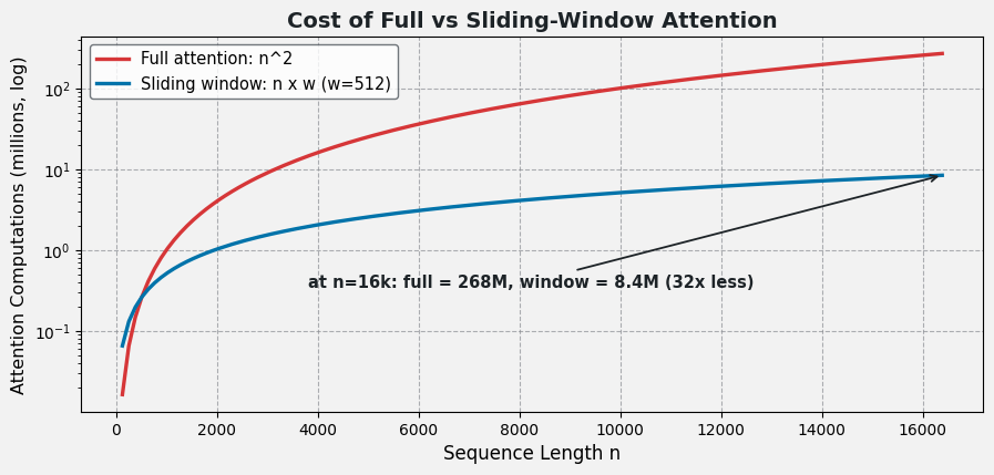
    Log-scale plot comparing n-squared full attention cost against n-times-w sliding window cost, with an annotation showing 32 times fewer computations at sequence length 16 thousand.

    Figure 2: At n = 16{,}384, full attention needs ~268M score computations versus ~8.4M for a 512-wide window, a 32x saving that grows with n.

    Used In: Longformer, BigBird (window + global + random blocks), and many long-document and code models where full O(n^2) attention is infeasible.


    Login to view more content
  • DL0027 Multi-Head Attention

    How does multi-head attention work in transformer architectures?

    Answer

    Multi-head attention runs several attention operations in parallel on different learned projections of the same input: Q, K, V are projected into h lower-dimensional subspaces (one per head), each head performs scaled dot-product attention independently, and the h outputs are concatenated and linearly re-projected by W^O. Each head can specialize in a different relationship (syntax, local neighborhoods, long-range links) so the combined representation is richer than any single attention map.

    (1) Split: Project d_{model}-dim Q, K, V into h heads of dimension d_k = d_{model} / h each.
    (2) Parallel Attention: Every head computes its own softmax-weighted sum; all heads run simultaneously, so total compute is comparable to one full-size head.
    (3) Merge: Concatenate the head outputs and apply output projection W^O back to d_{model}.

    Diagram of Q, K, V splitting into four parallel attention heads with different specializations, concatenating, and passing through an output projection to the model dimension.

    Figure 1: The MHA pipeline: split → parallel attention → concat → project; each head attends in its own subspace.

    Mathematical Formulation:
    \mathrm{MultiHead}(Q, K, V) = \mathrm{Concat}(\mathrm{head}_1, \dots, \mathrm{head}_h)\, W^O
    \mathrm{head}_i = \mathrm{Attention}(Q W_i^Q,\; K W_i^K,\; V W_i^V)

    Where:

    • W_i^Q, W_i^K, W_i^V \in \mathbb{R}^{d_{model} \times d_k} are the per-head projection matrices; h is the number of heads.
    • d_k = d_{model} / h is each head’s subspace dimension (e.g., 512-dim model with 8 heads → d_k = 64).
    • W^O \in \mathbb{R}^{h d_k \times d_{model}} mixes the concatenated heads back to the model dimension.
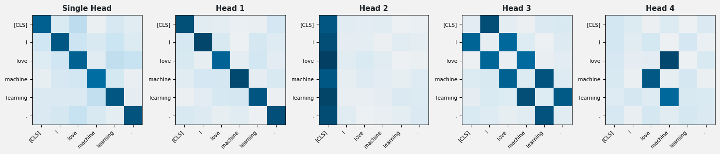
    Why Multiple Heads Help: A single softmax distribution must average every relationship into one map; separate heads let the model attend to different positions and relation types simultaneously. Empirically, heads specialize into recognizable patterns.

    Five attention heatmaps over the same sentence: one single-head map and four multi-head maps showing distinct patterns such as diagonal focus, CLS-column focus, local neighbor bands, and semantic links.

    Figure 2: Same input, four different attentions: heads specialize on position bands, special tokens, and semantic pairs that one head alone could not capture.


    Login to view more content