Tag: Transformer

  • DL0076 GQA: Grouped-Query Attention

    What is grouped-query attention (GQA), and why is it introduced?

    Answer

    Grouped-query attention splits the H query heads of a layer into H_{kv} groups and gives each group a single shared key head and value head, so the number of distinct K/V projections drops from H to H_{kv} while every query head keeps its own W_Q. It is the interpolation between two known extremes: H_{kv} = H is ordinary multi-head attention (MHA), and H_{kv} = 1 is multi-query attention (MQA). It exists because autoregressive decoding is memory-bandwidth bound, not compute bound: generating one token requires re-reading the entire KV cache from HBM, and that cache scales linearly with H_{kv}. MQA already fixed the bandwidth problem but lost quality and was unstable to train, so GQA was proposed to recover almost all of MQA’s decode speed at close to MHA quality by keeping a small number of K/V heads (typically 8). Nearly every major recent open-weight family ships with it, including Llama 3, where all sizes use 8 KV heads; the notable exception is DeepSeek-V2 and V3, which replace head sharing with multi-head latent attention.

    (1) The Bottleneck It Targets: the KV cache, not the weights, is what grows with batch size and context, and decode re-reads all of it per token, so shrinking it by H / H_{kv} directly raises arithmetic intensity and tokens per second.
    (2) A Dial Between Two Extremes: the lineage MHA → MQA → GQA is a single knob H_{kv}; 8 KV heads recovers most of the memory win of 1 while avoiding the quality drop that MQA shows on summarization and long-input tasks.
    (3) Cheap To Retrofit: an existing MHA checkpoint is converted by mean-pooling the K and V projections within each group and then uptraining on roughly 5% of the original pretraining tokens, so no full retrain is needed.
    (4) Set H_{kv} To The Tensor-Parallel Degree: with H_{kv} equal to the number of shards, each GPU owns exactly one KV head and nothing is replicated; a smaller H_{kv} forces the same K/V to be duplicated across shards and gives back part of the saving.
    (5) Almost No FLOP Change: the query projections and the QK^{\top} product are untouched, so prefill latency barely moves; GQA is a memory and bandwidth optimization, not a compute one.
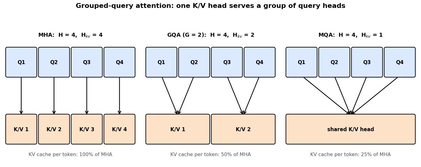
    Three panels each showing four query head boxes above their key/value heads: MHA has four separate KV heads, GQA with group size two has two KV heads each fed by two query heads, and MQA has one KV head shared by all four query heads

    Figure 1: The only structural change is how many distinct K/V heads exist; query heads are never merged, so each still has its own projection and its own attention pattern over the shared keys.

    Mathematical Formulation:
    H_{kv} = H / G
    g(i) = \lfloor i / G \rfloor
    M_{tok} = 2 L H_{kv} d_h b
    W_K^{(g)} = \frac{1}{G} \sum_{i \in \mathcal{G}_g} W_K^{(i)}

    Where:

    • H is the number of query heads, G the group size, and H_{kv} the resulting number of key/value heads; G = 1 recovers MHA and G = H recovers MQA.
    • i \in \{0,\ldots,H-1\} indexes query heads and g(i) is the KV head that head i reads, so heads are assigned to groups by contiguous blocks.
    • M_{tok} is the KV cache bytes per token, with L layers, head dimension d_h, bytes per element b, and the factor 2 covering K and V; total cache is M_{tok} times batch times sequence length.
    • \mathcal{G}_g is the set of query-head indices in group g, and the last line is the mean-pooling initialization used when converting an MHA checkpoint; the same averaging is applied to W_V.

    The payoff is easiest to see with a concrete configuration. A Llama-3-70B-shaped model has L = 80, H = 64, and d_h = 128; in FP16 that is 2.5 MiB per token of KV cache under MHA, 320 KiB under GQA with 8 KV heads, and 40 KiB under MQA. At a 32K context and batch size 1 those become 85.9 GB, 10.7 GB, and 1.34 GB. On a single H100 with 3.35 TB/s of HBM bandwidth, reading a 10.7 GB cache once costs roughly 3.2 ms per decoded token against roughly 26 ms for the 85.9 GB version; tensor parallelism divides both numbers, but the ratio is fixed by H_{kv} and does not improve with more hardware. That freed memory is also what lets a server hold many more concurrent sequences, which is usually a larger throughput win than the per-token latency itself.

    Log-scale bar chart of FP16 KV cache size at 32K context for a 70B-shaped model: MHA with 64 KV heads needs 85.9 GB, GQA with 8 KV heads needs 10.7 GB, and MQA with 1 KV head needs 1.34 GB, with a dashed line marking 80 GB of H100 HBM

    Figure 2: FP16 KV cache for one 32K-token sequence on an 80-layer, 64-head, 128-dim model. Under MHA the cache alone would consume an entire 80 GB H100 before any weights are loaded.

    PropertyMHAGQA (8 KV heads)MQA
    KV heads64 (one per query head)8 (group size 8)1 (shared by all)
    Cache per token (FP16)2.5 MiB320 KiB40 KiB
    Decode speedSlowest, bandwidth bound on the cacheClose to MQA at long contextFastest
    QualityReferenceWithin noise of MHA on most benchmarksMeasurable drop, notably on long-input summarization
    Tensor parallelismShards cleanlyShards cleanly when H_{kv} equals the shard countKV must be replicated on every shard
    Training stabilityStable baselineStable; uptrainable from an MHA checkpointReported instability at scale

    Login to view more content
  • DL0075 Attention Sink

    What is an attention sink, and why do models attend to the first token so heavily?

    Answer

    An attention sink is a token that a head dumps its attention mass onto when it has nothing relevant to retrieve, and in decoder-only LLMs that token is almost always the first one in the sequence (often the BOS token). Measured on a trained model, a middle-layer head can place well over half of its probability on that single position even though its value vector carries almost no task-relevant content. The cause is structural rather than semantic: softmax normalizes every attention row to sum to exactly 1, so a head has no way to say “attend to nothing” and must put the leftover mass somewhere. Causal masking makes the first token the only key visible from every query position, and it is the one token whose representation is not yet mixed with context, so training converges on it as the default no-op target. The model then reinforces the arrangement by growing massive activations and unusually large key norms at that position, which is why the sink shows up as an outlier in both attention maps and activation histograms.

    (1) Softmax Has No No-Op: the row constraint \sum_j \alpha_{ij} = 1 means an idle head still emits a full distribution, so the mass must land on some low-cost token.
    (2) Why The First Token Wins: under causal masking it is the only key every query can see, and it precedes all content, so it is both universally available and information-free, the ideal dumping ground.
    (3) The Sink Is Load-Bearing: it is not decorative; drop the first token from a sliding-window KV cache and perplexity jumps by one to two orders of magnitude, because every head loses its default target and redistributes mass onto real tokens.
    (4) Fingerprints Beyond Attention: the same position carries hidden-state outliers that widen activation ranges, which is a known headache for per-tensor quantization; vision transformers show the analogous effect by repurposing background patches as sinks.

    Log-scale bar chart of attention mass by key position for one head at query position 512: token 0 receives 0.42, tokens 1 to 3 receive 0.06, 0.03 and 0.02, three middle bins receive 0.07, 0.06 and 0.09, and the most recent 64 positions receive 0.25

    Figure 1: Illustrative single head at query position 512: the first token absorbs 0.42 of the mass, the most recent 64 positions share 0.25, and the roughly 444 middle positions split only 0.22, about 5\times 10^{-4} each.

    The cleanest way to read the sink is as a learned bias term smuggled into the softmax. Because the denominator sums over all visible keys, the only way for a head to shrink the weight it gives to real tokens is to inflate the score of some other key; the first token, whose value vector contributes near-zero to the output, is that escape valve. This also explains the standard fixes. Giving the softmax an explicit extra term in the denominator (the off-by-one softmax, or a learned per-head sink logit as used in some recent open-weight models such as OpenAI’s gpt-oss) lets attention rows sum to less than 1, so no real token needs to be sacrificed. Prepending dedicated register tokens achieves the same thing with ordinary softmax by supplying a scratch position, which is what cleaned up the noisy attention maps in vision transformers. Both changes must be present during pretraining: retrofitting them onto a model that already routes mass through token 0 changes the normalization the weights were trained under.

    Mathematical Formulation:
    s_{ij} = \frac{q_i^{\top} k_j}{\sqrt{d_k}}
    \alpha_{ij} = \frac{\exp(s_{ij})}{\sum_{m=1}^{i} \exp(s_{im})}
    \sum_{j=1}^{i} \alpha_{ij} = 1
    \tilde{\alpha}_{ij} = \frac{\exp(s_{ij})}{\exp(b_h) + \sum_{m=1}^{i} \exp(s_{im})}

    Where:

    • s_{ij} is the scaled dot-product score between query q_i and key k_j, with head dimension d_k.
    • \alpha_{ij} is the attention weight; i indexes query positions and j, m index key positions, restricted to m \leq i by causal masking, which is why j = 1 is the only key shared by every query.
    • The third line is the normalization constraint that creates the sink: no configuration of scores lets a head emit less than one unit of total mass.
    • b_h is a learned per-head sink logit added to the denominator, so \sum_j \tilde{\alpha}_{ij} can fall below 1; the off-by-one softmax is the special case b_h = 0, since \exp(0) = 1.
    Log-scale perplexity versus tokens streamed for three attention policies: dense attention rises past the 4096-token pretraining length, sliding-window attention jumps from about 10 to nearly 400 once the first token is evicted at 1024 tokens, and a window that retains 4 sink tokens stays flat near 10.5

    Figure 2: Illustrative streaming behavior: a plain sliding window collapses the moment the first token leaves the KV cache, while retaining a handful of sink tokens alongside the window keeps perplexity flat far beyond the pretraining length.

    ApproachWhat It ChangesTraining CostWhen to Reach for It
    Dense AttentionNothing; the sink stays at token 0 and is never evictedNoneShort contexts where the full KV cache fits
    Keep First k Tokens (StreamingLLM)Cache policy only: pin the first 4 tokens plus a sliding windowNone, works on an already-trained modelStreaming or long-running serving with a fixed cache budget
    Register or Sink TokensPrepends learnable scratch tokens that heads can dump ontoPretraining or substantial fine-tuningNew models, and ViTs whose attention maps must stay interpretable
    Learned Sink Logit / Softmax Off-by-OneExtra denominator term so a row can sum to less than 1Must be present from pretrainingNew architectures, especially where activation outliers hurt quantization

    Login to view more content
  • DL0067 BERT VS GPT Pretraining

    How does BERT’s pre-training objective differ from GPT’s?

    Answer

    BERT is trained primarily with masked language modeling: selected input tokens are corrupted, and a bidirectional encoder predicts the original tokens from visible context on both sides. GPT uses causal language modeling: a decoder predicts each next token using only earlier tokens, enforced by a triangular attention mask. MLM supplies loss only at selected positions and creates a corruption mismatch between pre-training and ordinary inputs, whereas causal modeling supplies a target at nearly every position and matches left-to-right generation. Original BERT also used next sentence prediction, while standard GPT pre-training relies on the autoregressive token objective rather than NSP.

    (1) Context Visibility: BERT’s visible tokens attend bidirectionally; GPT position t cannot attend to positions later than t.
    (2) Prediction Targets: BERT reconstructs a selected masked subset, while GPT shifts the sequence and predicts the next token at each usable position.
    (3) Downstream Bias: BERT naturally supports full-context understanding, whereas GPT’s objective directly trains open-ended autoregressive generation; either family can be adapted beyond that bias.

    Side-by-side BERT masked-language-modeling and GPT causal-language-modeling pre-training objectives.

    Figure 1: BERT reconstructs selected corrupted tokens from two-sided context, while GPT predicts the next token at every step from a left-only prefix.

    Mathematical Formulation:
    \mathcal{L}_{\mathrm{BERT}}=-\sum_{i\in\mathcal{M}}\log p(x_i\mid x_{\setminus\mathcal{M}})
    \mathcal{L}_{\mathrm{GPT}}=-\sum_{t=1}^{T}\log p(x_t\mid x_{1:t-1})

    Where:

    • \mathcal{L}_{\mathrm{BERT}} and \mathcal{L}_{\mathrm{GPT}} are the masked and causal language-modeling losses.
    • \mathcal{M} is BERT’s selected target set and i\in\mathcal{M} indexes one target token x_i.
    • x_{\setminus\mathcal{M}} denotes BERT’s visible corrupted context outside the selected targets, and p(x_i\mid x_{\setminus\mathcal{M}}) is the reconstruction probability.
    • t\in\{1,\ldots,T\} indexes a GPT target position, T is sequence length, and x_{1:t-1} is the preceding token prefix.
    • p(x_t\mid x_{1:t-1}) is the next-token probability and \log converts each probability into a log-likelihood term.
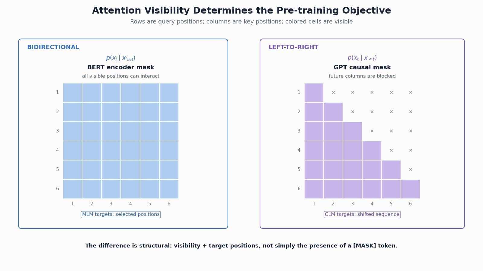
    BERT bidirectional and GPT causal attention matrices with their respective training target positions.

    Figure 2: Attention visibility explains the objective difference: BERT uses a full visible-context matrix, while GPT uses a lower-triangular causal matrix.


    Login to view more content
  • DL0066 BERT

    What is BERT and how is it used in NLP tasks?

    Answer

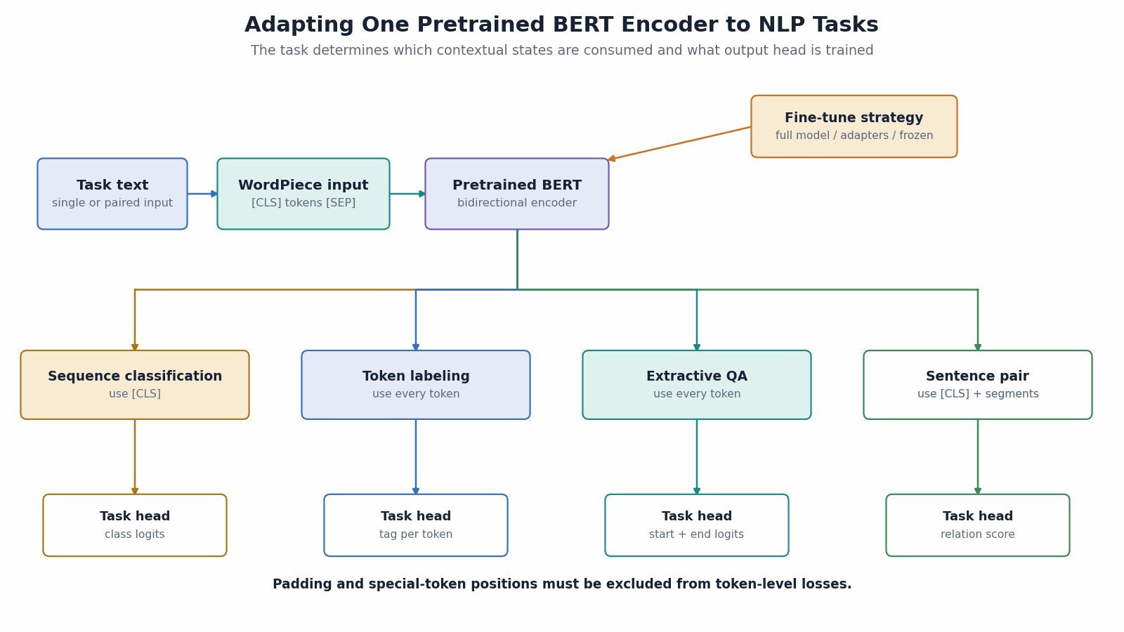
    BERT is a Transformer encoder pretrained to build bidirectional contextual representations of text. Its input combines token, segment, and positional embeddings, and every encoder layer lets each unmasked token attend to context on both sides. Original BERT is pretrained with masked language modeling and next sentence prediction, then adapted by adding a small task head and fine-tuning the whole model or using its representations. The [CLS] output supports sequence-level tasks, token outputs support tagging, and paired start/end scores support extractive question answering.

    (1) Bidirectional Encoder: Unlike a causal decoder, BERT‘s self-attention normally uses both left and right context for every visible input token.
    (2) Pre-Training: Original BERT predicts selected masked tokens and also trains an NSP classifier; later BERT-family models often modify or remove NSP.
    (3) Task Adaptation: A lightweight output head maps contextual states to sequence labels, token labels, sentence-pair scores, or answer spans.

    BERT input embeddings and bidirectional Transformer encoder producing contextual token representations.

    Figure 1: BERT combines token, segment, and position embeddings, processes them with bidirectional encoder layers, and exposes contextual outputs.

    Mathematical Formulation:
    H=\mathrm{Encoder}(E_{\mathrm{token}}+E_{\mathrm{segment}}+E_{\mathrm{position}})
    \mathcal{L}_{\mathrm{MLM}}=-\sum_{i\in\mathcal{M}}\log p(x_i\mid x_{\setminus\mathcal{M}})

    Where:

    • E_{\mathrm{token}}, E_{\mathrm{segment}}, and E_{\mathrm{position}} are token, segment, and positional embedding matrices for the input sequence.
    • \mathrm{Encoder} is the bidirectional Transformer stack and H contains one contextual vector per input position.
    • \mathcal{L}_{\mathrm{MLM}} is masked-language-modeling loss and \mathcal{M} is the selected set of prediction positions.
    • i\in\mathcal{M} indexes one selected target, x_i is its original token, and x_{\setminus\mathcal{M}} denotes the visible corrupted context outside the selected targets.
    • p(x_i\mid x_{\setminus\mathcal{M}}) is the model probability assigned to the original target token given visible context.
    BERT fine-tuning flowchart for classification, token labeling, question answering, and sentence pairs.

    Figure 2: The same pretrained encoder can be adapted with small heads that consume either [CLS], every token state, or start/end span scores.


    Login to view more content
  • DL0063 Transformer Variable Length Sequences

    How does the Transformer handle variable-length sequences?

    Answer

    A Transformer can process different sequence lengths because self-attention is defined over whatever number of tokens is supplied, up to the model’s context limit. For efficient batching, implementations usually pad sequences to a common length or group examples of similar lengths, then apply a padding mask so valid queries cannot attend to padded keys and values. Decoder-style models also add a causal mask that blocks future positions, while positional encodings identify token order within each sequence. Padded query outputs and losses must be ignored, and computation still scales with the padded batch length rather than only the number of valid tokens.

    (1) Batch Construction: Sequences are dynamically padded to the longest item in a batch, bucketed by length, or packed by specialized kernels to reduce wasted work.
    (2) Attention Masking: A key-padding mask removes padded keys and values from attention; causal models combine it with a triangular future mask.
    (3) Length Boundary: Variable length does not mean unlimited length: positional support, memory, and the configured context window impose a maximum.

    Variable-length token sequences padded into one batch with key-padding and causal attention masks.

    Figure 1: Unequal token sequences become a rectangular batch; masking separates valid context, padding, and future positions.

    Mathematical Formulation:
    \mathrm{Attention}(Q,K,V)=\mathrm{softmax}\!\left(\frac{QK^\top}{\sqrt{d_k}}+M_{\mathrm{pad}}+M_{\mathrm{causal}}\right)V
    M_{ij}\in\{0,-\infty\}

    Where:

    • Q, K, and V are query, key, and value matrices, and d_k is the key width used for score scaling.
    • M_{\mathrm{pad}} assigns -\infty to padded key positions so their softmax probabilities become zero.
    • M_{\mathrm{causal}} assigns -\infty when key index j is later than query index i; encoder-only models normally omit this mask.
    • M_{ij} denotes one combined mask entry and is either 0 for an allowed connection or -\infty for a blocked connection.
    • B is batch size and L_{max} is padded sequence length, giving a dense token tensor of shape B\times L_{max}.
    Transformer variable-length processing flowchart from tokenization through masks and output cleanup.

    Figure 2: A practical variable-length pipeline: tokenize, bucket or pad, build masks, run attention, then ignore padded outputs or continue autoregressive generation.


    Login to view more content
  • DL0061 Channel and Spatial Attention

    Explain channel attention and spatial attention in CNNs. What information does each mechanism model?

    Answer

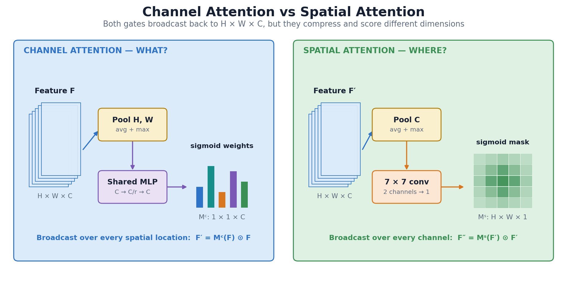
    Channel attention learns which feature channels are important, answering what semantic responses should be emphasized. It compresses spatial dimensions into channel descriptors, transforms them with a small gating network, and multiplies the resulting weights into the feature tensor. Spatial attention learns where informative regions occur by compressing or projecting the channel dimension and producing an H\times W mask. Modules such as SE use channel attention, while CBAM applies channel attention followed by spatial attention to refine both feature type and location.

    (1) Channel Gate: Global pooling summarizes each channel; an MLP or 1D convolution captures inter-channel dependence and outputs C multiplicative weights.
    (2) Spatial Gate: Average/max pooling or learned projection across channels produces spatial descriptors that a convolution maps to one H\times W attention mask.
    (3) Residual Placement: Attention usually modulates an existing feature tensor and is often inserted inside a residual block; sigmoid gates reweight rather than replace the underlying features.

    Channel attention and spatial attention mechanisms with tensor reductions and broadcast multiplication.

    Figure 1: Parallel tensor-shape explanation of what channel attention selects and where spatial attention focuses.

    Mathematical Formulation:
    M_c(F)=\sigma\!\left(\mathrm{MLP}(\mathrm{AvgPool}_{hw}(F))+\mathrm{MLP}(\mathrm{MaxPool}_{hw}(F))\right)
    M_s(F)=\sigma\!\left(f^{7\times7}([\mathrm{AvgPool}_{c}(F);\mathrm{MaxPool}_{c}(F)])\right)

    Where:

    • F\in\mathbb{R}^{H\times W\times C} is the input feature map with height H, width W, and C channels.
    • M_c(F)\in\mathbb{R}^{1\times1\times C} is the channel mask; spatial average/max pooling and the shared \mathrm{MLP} produce channel logits.
    • M_s(F)\in\mathbb{R}^{H\times W\times1} is the spatial mask; channel pooling outputs are concatenated by [\,;\,] and filtered by f^{7\times7}.
    • \sigma is the sigmoid function; M_c broadcasts over H,W, while M_s broadcasts over C.
    Sequential CBAM channel-then-spatial attention flowchart.

    Figure 2: CBAM data flow from input feature through channel gating, spatial gating, residual refinement, and output.


    Login to view more content
  • DL0056 FlashAttention

    Explain FlashAttention. Why can it compute exact attention faster while using less memory?

    Answer

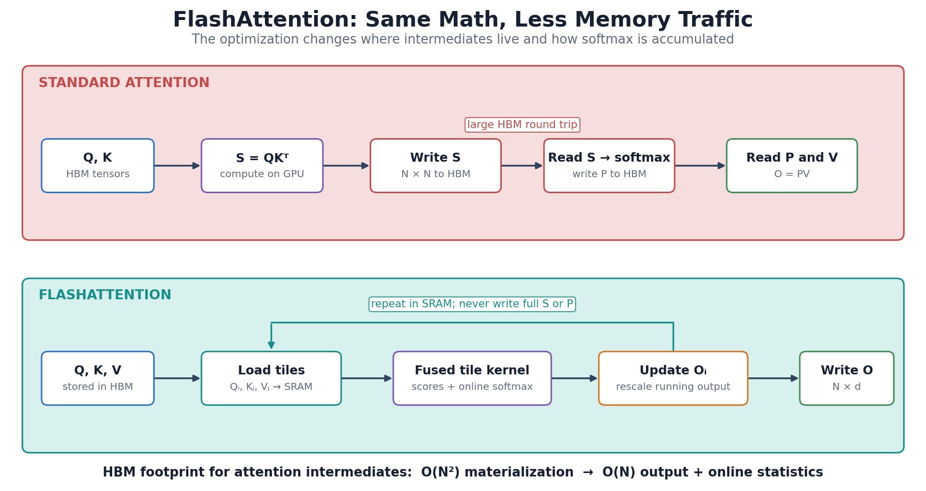
    FlashAttention is an exact, IO-aware implementation of scaled dot-product attention. Instead of materializing the full N\times N score and probability matrices in high-bandwidth memory (HBM), it loads blocks of Q, K, and V into fast on-chip SRAM, computes attention block by block, and maintains online softmax statistics. Tiling reduces expensive HBM reads and writes, while recomputation during the backward pass can be cheaper than storing large intermediates. The mathematical result matches standard attention up to normal floating-point differences; the speedup comes from changing the execution schedule, not from approximating attention.

    (1) IO Awareness: The kernel is organized around the GPU memory hierarchy so most score computation and softmax updates happen in SRAM.
    (2) Online Softmax: A running row maximum and normalization sum allow each K,V tile to update the output without retaining previous score blocks.
    (3) Exact Result: All query-key interactions are evaluated; causal masking, dropout, and backward gradients are fused into specialized kernels rather than approximated.

    Comparison of standard attention and FlashAttention data movement through HBM and SRAM.

    Figure 1: IO comparison showing why avoiding N×N intermediate writes makes FlashAttention faster and more memory efficient.

    Mathematical Formulation:
    m_i^{(t)}=\max\!\left(m_i^{(t-1)},\max_j S_{ij}^{(t)}\right)
    \ell_i^{(t)}=e^{m_i^{(t-1)}-m_i^{(t)}}\ell_i^{(t-1)}+\sum_j e^{S_{ij}^{(t)}-m_i^{(t)}}

    Where:

    • t indexes key/value tiles, i indexes a query row, and j indexes keys inside tile t.
    • S_{ij}^{(t)}=Q_iK_j^T/\sqrt d is the scaled score between query row Q_i and key row K_j, with head width d.
    • m_i^{(t)} is the running row maximum after tile t, initialized with m_i^{(0)}=-\infty.
    • \ell_i^{(t)} is the running softmax denominator, initialized with \ell_i^{(0)}=0; the exponential factors rescale earlier partial sums when the maximum changes.
    FlashAttention tiled online-softmax flowchart for one query block.

    Figure 2: Blockwise FlashAttention loop with running maximum, normalization, output rescaling, and final HBM write.


    Login to view more content
  • DL0055 Vision Transformer

    Explain the Vision Transformer (ViT). How does it convert an image into a class prediction?

    Answer

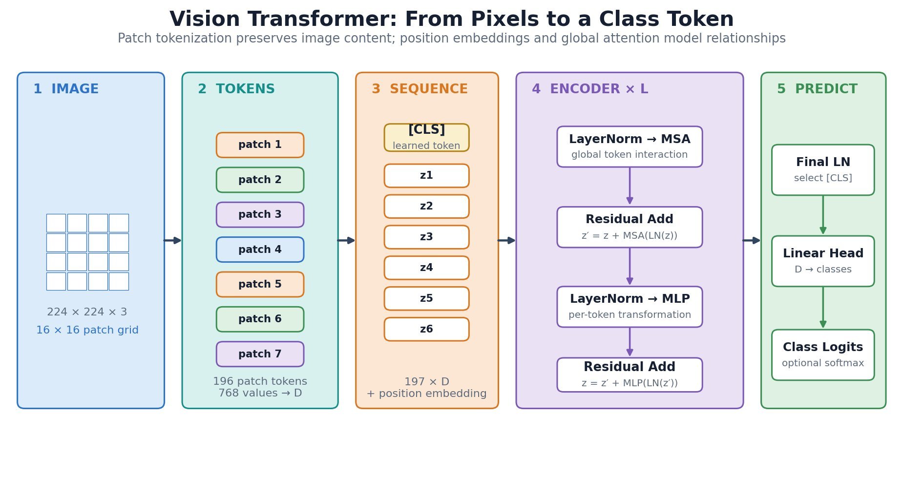
    A Vision Transformer converts an image into a sequence of fixed-size patch tokens and processes them with a Transformer encoder. A learned class token is prepended, positional embeddings preserve patch order, and global self-attention lets every patch exchange information with every other patch. After the encoder stack, the class-token representation is passed to a prediction head. Compared with a CNN, a ViT has weaker built-in locality and translation bias, but it can model long-range interactions directly and scales effectively with data and compute.

    (1) Tokenization: An image of shape H\times W\times C is divided into N=(H/P)(W/P) non-overlapping P\times P patches; each flattened patch is projected to width D.
    (2) Global Context: Multi-head self-attention mixes information across all patch positions, while residual connections and MLP sublayers refine each token.
    (3) Classification: A learned [CLS] token aggregates evidence across the encoder stack; its final state is normalized and mapped to class logits.

    Vision Transformer architecture from image patchification through token encoding and classification.

    Figure 1: ViT architecture with tensor shapes, patch tokenization, the Transformer encoder stack, and the classification path.

    Mathematical Formulation:
    z_0=[x_{\mathrm{cls}};x_p^1E;x_p^2E;\ldots;x_p^NE]+E_{\mathrm{pos}}
    \mathrm{Attention}(Q,K,V)=\mathrm{softmax}\!\left(\frac{QK^T}{\sqrt{d_h}}\right)V

    Where:

    • z_0 is the initial token sequence supplied to the Transformer encoder.
    • x_{\mathrm{cls}} is the learned class token, and x_p^i is flattened image patch i.
    • E\in\mathbb{R}^{P^2C\times D} projects each P\times P\times C patch to width D, while E_{\mathrm{pos}} supplies positional embeddings.
    • N=(H/P)(W/P) is the patch count for an image of height H, width W, and channel count C.
    • Q, K, and V are query, key, and value matrices; d_h is the per-head query/key width.
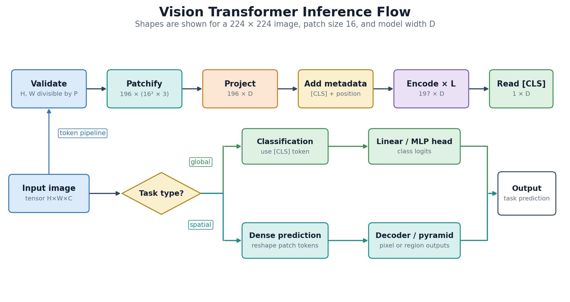
    Vision Transformer inference flowchart showing the ordered transformation from pixels to class logits.

    Figure 2: ViT inference flow from image validation and patch embedding to encoder processing and class prediction.


    Login to view more content
  • DL0054 Deformable Attention

    What is Deformable Attention and how does it reduce computational complexity for object detection tasks?

    Answer

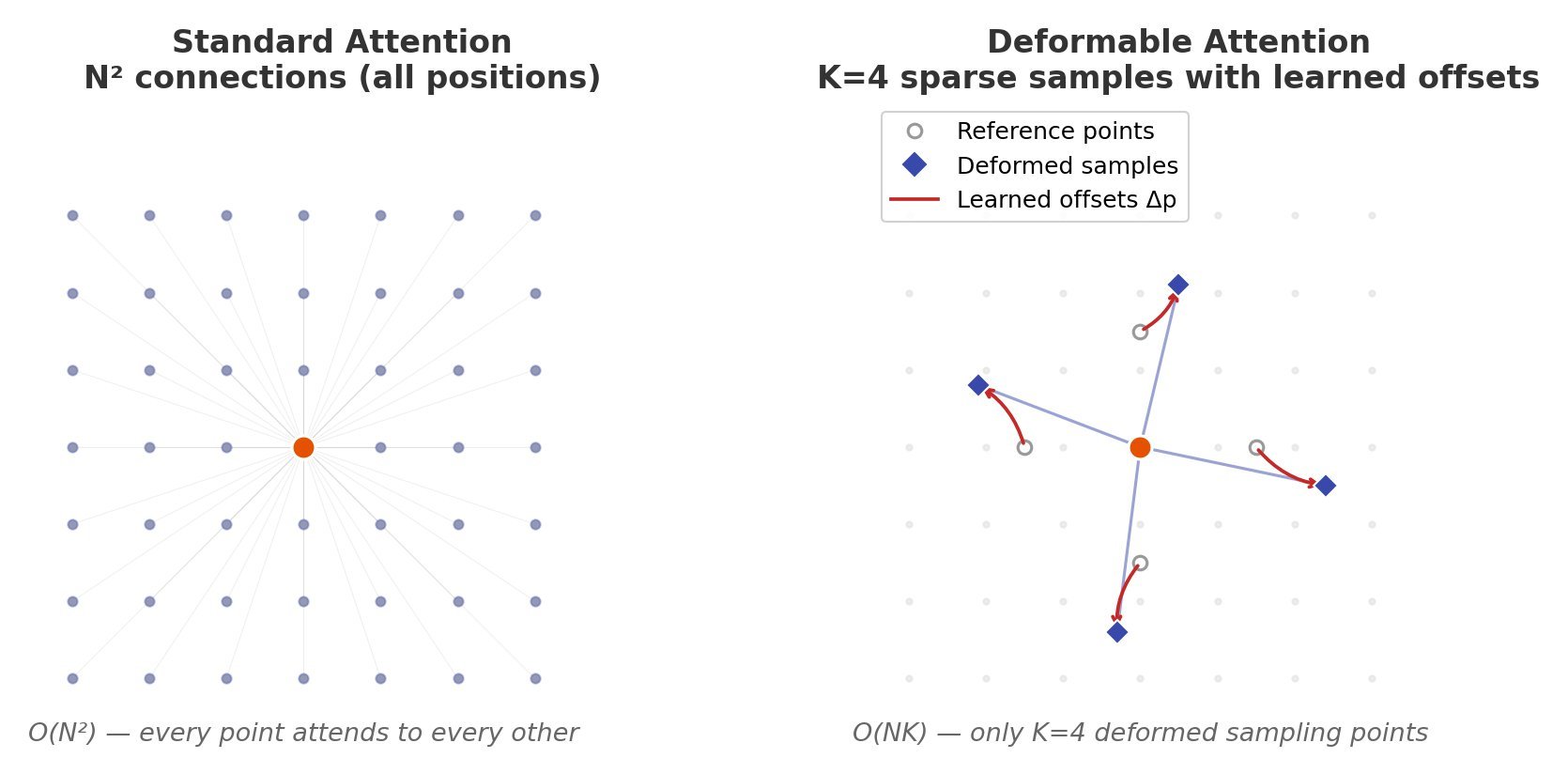
    Deformable Attention is a sparse attention mechanism that learns dynamic sampling locations instead of attending to all spatial positions uniformly. It uses learned 2D offsets from reference points to sample only the most relevant features, reducing complexity from O(N^2) to O(NK) where K is a small constant (typically 4). This makes it ideal for high-resolution feature maps in object detection where full attention is computationally prohibitive — for a 1024×1024 feature map (N \approx 10^6 positions), standard attention requires ~1T operations per head while deformable attention needs only ~4M.

    (1) Sparse Sampling: Instead of computing attention over all N \times N positions, deformable attention samples only K reference points per query, typically K=4 or 8, reducing the key-value set from N to K.
    (2) Learned Offsets: The model predicts \Delta p_{mk} offsets from each reference point p_k using a lightweight linear layer on query features, requiring only O(NC) additional computation where C is channel dimension.
    (3) Bilinear Interpolation: When offsets point to non-integer locations, bilinear interpolation computes feature values from the 4 nearest pixels, enabling sub-pixel precision sampling without modifying the feature map.

    Sparse Sampling Locations Diagram

    Figure 1: Deformable attention learns K=4 sampling offsets per query point instead of dense N×N attention

    Mathematical Formulation:
    y(p) = \sum_{m=1}^{M} W_m \left[ \sum_{k=1}^{K} A_{mk} \cdot W_m' x(p + p_k + \Delta p_{mk}) \right]

    Where:

    •  p is the reference position (query location on the feature map)
    •  M is the number of attention heads
    •  K is the number of sampled keys per head (typically 4)
    •  p_k are fixed reference offsets (uniformly initialized)
    •  \Delta p_{mk} are learned deformable offsets (2D, predicted per head per key)
    •  A_{mk} is the attention weight (normalized, not from softmax over all positions)
    •  W_m, W_m' are projection matrices for each head
    Complexity Comparison Chart

    Figure 2: Complexity comparison shows O(NK) grows linearly while O(N²) becomes prohibitive for large feature maps

    The offsets \Delta p_{mk} are predicted by a linear projection from query features: \Delta p_{mk} = W_\text{offset} \cdot q_m(p), where W_\text{offset} \in \mathbb{R}^{C \times 2K}. The attention weights A_{mk} are computed via a separate softmax over only K elements, not the full N positions. In Deformable DETR, multi-scale deformable attention extends this to sample across multiple feature map resolutions simultaneously, enabling the model to capture both small and large objects efficiently.


    Login to view more content
  • DL0053 Gated Attention

    What is Gated Attention and how does it improve transformer architectures over standard scaled dot-product attention?

    Answer

    Gated Attention (arXiv:2505.06708) applies a head-specific sigmoid gate after Scaled Dot-Product Attention (SDPA) to dynamically modulate attention output. Unlike standard attention where all heads contribute equally, gated attention introduces query-dependent sparse gating that suppresses irrelevant heads and activates only salient ones. This mitigates the attention sink problem where standard transformers concentrate disproportionate attention on the first few tokens, and enhances long-context extrapolation by maintaining diverse attention patterns across sequence lengths.

    (1) Post-SDPA Gating: The gate is applied after SDPA computation, not before — each attention head h_i is multiplied by a sigmoid gate g_i = \sigma(W_g \cdot q_i) where W_g is a head-specific projection.
    (2) Sparsity Induction: The sigmoid gate produces values in [0, 1], and empirical measurements show mean gate activation of ~0.116, meaning most heads are heavily suppressed — introducing beneficial sparsity without hard pruning.
    (3) Attention Sink Mitigation: Standard attention allocates ~46.7% of attention mass to the first token; gated attention reduces this to ~4.8%, distributing attention more uniformly across tokens.

    Gated Attention Mechanism Diagram

    Figure 1: Gated attention applies a head-specific sigmoid gate after SDPA to modulate attention output before the residual connection

    Mathematical Formulation:
    \text{GatedAttn}(Q, K, V) = \text{Concat}(g_1 \odot h_1, \ldots, g_H \odot h_H) W_O
    g_i = \sigma(W_g^{(i)} \cdot q_i + b_g^{(i)})

    Where:

    •  h_i = \text{SDPA}(q_i, k_i, v_i) is the output of the i-th attention head
    •  g_i \in [0, 1] is the head-specific gate score
    •  W_g^{(i)} \in \mathbb{R}^{d_k \times 1} is a learned projection from query to scalar gate
    •  \sigma is the sigmoid function
    •  \odot denotes element-wise multiplication
    •  W_O is the standard output projection
    Gate Activation Distribution

    Figure 2: Gate activation distribution across 8 attention heads shows heavy suppression (mean ~0.116) with sparse high-activation regions

    The gate projection W_g^{(i)} adds only O(d_k) parameters per head — a negligible overhead of ~0.1% of total model parameters — yet significantly improves long-context performance. On the RULER benchmark at 128K context length, gated attention improves needle-in-haystack retrieval accuracy from ~72% to ~94% compared to standard attention.


    Login to view more content