Tag: Transformer

  • DL0052 Rotary Positional Embedding

    What is Rotary Positional Embedding (RoPE)?

    Answer

    Rotary Positional Embedding (RoPE) encodes position by rotating each pair of query/key dimensions by an angle proportional to the token’s position, instead of adding a position vector. Because a rotation at position m composed with one at position n depends only on the difference, the attention dot product between tokens automatically reflects their relative distance, with no learned parameters and good length generalization. RoPE is the default in GPT-NeoX, LLaMA, PaLM, Qwen, and most modern LLMs.

    (1) Geometric Encoding: Each 2D slice of a query or key vector is rotated by m\theta_i, where m is the token position and \theta_i the per-dimension frequency.
    (2) Relative From Absolute: The dot product of two rotated vectors depends on (m - n)\theta_i only: absolute rotations yield relative-position attention.
    (3) Parameter-Free and Efficient: No embedding table, no attention bias, just a fixed trigonometric transform applied to Q and K.

    Mathematical Formulation:
    f(x, m) = \begin{pmatrix} \cos(m\theta) & -\sin(m\theta) \\ \sin(m\theta) & \cos(m\theta) \end{pmatrix} \begin{pmatrix} x_1 \\ x_2 \end{pmatrix}
    \theta_i = 10000^{-2i/d}

    Where:

    • m is the token’s absolute position in the sequence; x_1, x_2 are one 2D pair of the query/key vector.
    • \theta_i is the rotation frequency of the i-th dimension pair, geometrically decreasing across pairs so low dimensions capture short-range and high dimensions long-range offsets.
    Line chart of attention similarity versus relative token distance, with RoPE similarity decaying smoothly as distance grows while sinusoidal absolute positional encoding stays flat.

    Figure 1: Similarity vs relative distance: RoPE decays smoothly with distance (a built-in recency prior), while sinusoidal absolute PE stays roughly flat.

    Why It Won: RoPE is shift-invariant (the same rotation rule works at any position), adds zero parameters or memory, and, unlike learned absolute embeddings, degrades gracefully beyond the training length, which is why context-extension methods (NTK scaling, YaRN) all build on rescaling its frequencies.


    Login to view more content
  • DL0045 Dimension in FFN

    In Transformers, why does the feed-forward network expand the hidden dimension (e.g.,  d_{\text{model}} → 4 d_{\text{model}} ) before reducing it back?

    Answer

    The FFN expands each token’s representation from d_{\text{model}} to 4 d_{\text{model}} to create a wide nonlinear workspace: in the higher-dimensional space the activation function can carve out far richer feature combinations than the residual stream’s width allows. It then projects back down so the result matches the residual stream for the skip connection and the next sub-layer. It is a bottleneck design that buys expressiveness where it is cheap while keeping the inter-layer interface narrow.

    (1) Extra Capacity: The wider hidden layer holds more features; the FFN is where most of a block’s parameters (8 d^2, about two-thirds) live.
    (2) Nonlinear Mixing: The activation (ReLU/GELU/SwiGLU) acts in the expanded space, letting the network represent sparse, high-order interactions that a d-wide layer cannot.
    (3) Projection Back: Returning to d_{\text{model}} keeps residual compatibility and a uniform interface across all layers.

    Mathematical Formulation:
    \mathrm{FFN}(x) = W_2\, \sigma(W_1 x + b_1) + b_2

    Where:

    • x \in \mathbb{R}^{d_{\text{model}}} is the per-token input from the residual stream.
    • W_1 \in \mathbb{R}^{4 d_{\text{model}} \times d_{\text{model}}} expands the dimension, \sigma is the nonlinearity, and W_2 \in \mathbb{R}^{d_{\text{model}} \times 4 d_{\text{model}}} projects back down.
    Feed-forward network flow: input of width d-model expands through linear W1 to 4 times d-model, passes an activation, then linear W2 reduces it back to d-model output.

    Figure 1: The FFN hourglass: expand d \to 4d, activate in the wide space, reduce 4d \to d to rejoin the residual stream.

    Empirical Note: The 4x factor dates to the original Transformer and was kept by BERT/GPT because it reliably improves loss; modern SwiGLU models (LLaMA) use ~2.7x with three matrices so the parameter count stays comparable.


    Login to view more content
  • DL0044 Multi-Query Attention

    What is Multi-Query Attention in transformer models?

    Answer

    Multi-Query Attention (MQA) is a variant of multi-head attention where all query heads share a single key and value projection instead of each head owning its own K/V. The KV cache therefore stores one K/V pair per token rather than one per head, shrinking cache memory and bandwidth by a factor of h, which directly speeds up autoregressive decoding, usually with only a minor quality cost.

    (1) Structure: Queries are still projected into h distinct heads, but all of them attend against one shared K and one shared V.
    (2) Cache Savings: The per-token KV cache drops from O(n \cdot h \cdot d_k) to O(n \cdot d_k), hx smaller.
    (3) Trade-off: Slightly less expressive than full MHA (one key/value “view” of the sequence), which GQA later interpolates by sharing K/V across small groups of heads.

    Mathematical Formulation:
    \mathrm{head}_i = \mathrm{softmax}\!\left(\frac{Q_i K_{\text{shared}}^{\top}}{\sqrt{d_k}}\right) V_{\text{shared}}
    \mathrm{Cache}_{\text{MQA}} = \frac{1}{h}\,\mathrm{Cache}_{\text{MHA}}

    Where:

    • Q_i is the query of head i \in \{1, \ldots, h\}; K_{\text{shared}}, V_{\text{shared}} are the single key/value projections used by all heads.
    • d_k is the head dimension and h the number of query heads.
    Side-by-side diagram of multi-head attention with separate query, key, and value boxes per head versus multi-query attention with many query heads converging on one shared key and value box.

    Figure 1: MHA gives every head its own K and V; MQA keeps multiple query heads but shares one K and one V across all of them.

    Why Decoding Gets Faster: Autoregressive inference is memory-bandwidth bound: every generated token must read the entire KV cache. An hx smaller cache means hx less data movement per step, which is why MQA (and its successor GQA, used in LLaMA-2/3) is standard in serving-oriented LLMs.


    Login to view more content
  • DL0043 KV Cache

    What is KV Cache in transformers, and why is it useful during inference?

    Answer

    The KV cache stores the key and value vectors of all previously generated tokens so that autoregressive decoding never recomputes them. At each step the model computes Q, K, V only for the new token, appends K and V to the cache, and attends over the cached history, turning each decoding step from an O(n^2 d) full recompute into an O(n d) lookup, at the price of O(n) growing memory.

    (1) What Is Cached: Per layer, the projected keys and values K_{1:t}, V_{1:t} of every past token; they never change once computed, so recomputing them is pure waste.
    (2) Why It Helps: With causal masking, token t attends to exactly K_{1:t}, V_{1:t}; caching reduces each step to one new query against a read-only cache.
    (3) The Cost: Memory grows linearly (2 \cdot n \cdot d values per layer for K and V, O(L \cdot n \cdot d) across L layers) and becomes the inference bottleneck for long contexts and large batches.

    Mathematical Formulation:
    \mathrm{Attention}(q_t, K_{1:t}, V_{1:t}) = \mathrm{softmax}\!\left(\frac{q_t K_{1:t}^{\top}}{\sqrt{d_k}}\right) V_{1:t}
    \mathrm{Memory}_{\text{cache}} = 2 \cdot L \cdot n \cdot d_{\text{model}} \;\; \text{values}

    Where:

    • q_t is the query of the current token t; K_{1:t}, V_{1:t} are the cached keys and values for tokens 1 \ldots t.
    • d_k is the per-head key dimension, d_{\text{model}} the model width, and L the number of layers; the factor 2 counts K and V buffers separately.
    Two-panel diagram of attention without cache, recomputing a full query matrix each step, versus with cache, computing only the new token's query and reusing cached keys and values.

    Figure 1: Without cache every step recomputes the full Q, K, V; with cache only the new token’s query is computed while cached K/V (purple) supply the history.

    Practical Note: During training the full sequence is processed in parallel so the cache does not apply; it is an inference-only optimization, and its size is why long-context serving is memory-bound rather than FLOP-bound.


    Login to view more content
  • DL0042 Attention Computation

    Please break down the computational cost of attention.

    Answer

    Attention cost splits into a linear-in-n term from projections and a quadratic-in-n term from pairwise interactions. For sequence length n and model dimension d, the total is O(n d^2 + n^2 d): projections dominate for short sequences, while the n \times n score matrix dominates once n grows past d.

    (1) Q/K/V + Output Projections: Four d \times d GEMMs over n tokens: O(n d^2), linear in sequence length.
    (2) Score Matrix QK^\top and Value Mixing AV: Pairwise n \times n work: O(n^2 d), the quadratic bottleneck.
    (3) Softmax: Elementwise over n^2 entries: O(n^2), cheap FLOPs but the n \times n matrix drives memory traffic.

    Mathematical Formulation (one attention layer, h heads, d_k = d_v = d/h):
    \mathrm{Cost}_{\text{proj}} = O(n\, d^2)
    \mathrm{Cost}_{\text{scores}} = O(n^2\, d_k \cdot h) = O(n^2 d)
    \mathrm{Cost}_{\text{total}} = O\!\left(n^2 d + n\, d^2\right)

    Where:

    • n is the sequence length, d the model (hidden) dimension, and h the number of heads.
    • Q, K \in \mathbb{R}^{n \times d_k} form scores S = QK^\top \in \mathbb{R}^{n \times n}; attention weights A = \mathrm{softmax}(S / \sqrt{d_k}) mix values V \in \mathbb{R}^{n \times d_v} via O = AV.
    • Multi-head attention costs the same as single-head in big-O: per-head dimensions scale as d/h, so the h heads sum back to d.
    Log-log plot of attention and projection FLOPs versus sequence length at hidden dimension 512, with the quadratic attention term overtaking the linear projection term near n equals 512.

    Figure 1: Log-log cost curves at d = 512: projection O(n d^2) leads at short lengths, attention O(n^2 d) takes over near n \approx d and dominates at long context.

    Regimes: Short sequences (n \ll d): the n d^2 projection term dominates. Long sequences (n \gg d): the n^2 d interaction term dominates; the two balance around n \approx d.


    Login to view more content
  • DL0041 Hierarchical Attention

    Could you explain the concept of hierarchical attention in transformer architectures?

    Answer

    Hierarchical attention applies self-attention at multiple levels of granularity instead of one flat pass over all tokens: first local attention within segments (words inside a sentence, frames inside a shot), then global attention across the aggregated segment representations (sentences inside a document). This mirrors the natural structure of long inputs, cuts the quadratic cost dramatically, and yields interpretable focus at each level.

    (1) Local Level (Fine-Grained): Each segment runs its own self-attention over its tokens, producing one segment embedding; cost grows with segment length, not document length.
    (2) Global Level (Coarse-Grained): The segment embeddings attend over each other, producing a document-level representation.
    (3) Efficiency Gain: A document of n tokens split into s segments of m tokens costs O(s m^2 + s^2) in attention entries instead of O(n^2), a large saving when m \ll n.

    Two-level hierarchy diagram: word tokens attend inside sentence segments, sentence embeddings then attend globally to form a document embedding.

    Figure 1: Two attention levels: local attention inside each segment, then global attention over segment embeddings to form the document representation.

    Mathematical Formulation (cost for n = s × m tokens):
    \text{Flat:}\quad \mathrm{Cost} \propto n^2
    \text{Hierarchical:}\quad \mathrm{Cost} \propto \underbrace{s\, m^2}_{\text{local}} + \underbrace{s^2}_{\text{global}} \ll n^2

    Where:

    • n is the total token count, split into s segments of m tokens each (n = s \cdot m).
    • The local term runs s independent m \times m attentions; the global term runs one s \times s attention over segment embeddings.

    Example (Document Classification): With n = 4096 tokens as s = 64 sentences of m = 64 words, flat attention scores 16.8\text{M} pairs, while hierarchical attention scores only 64 \cdot 64^2 + 64^2 \approx 0.27\text{M}, roughly 60x fewer pairs.


    Login to view more content
  • DL0040 Attention Mask

    What is the role of masking in attention?

    Answer

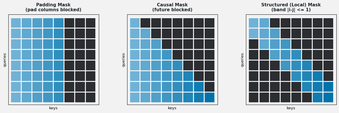
    Masking controls which positions attention is allowed to see. Before softmax, disallowed score entries are set to -\infty (a very large negative number), so their attention weights become exactly zero. This one mechanism serves three jobs: preventing future leakage in autoregressive decoding, ignoring padding tokens in batched inputs, and enforcing task structure such as local neighborhoods or blocked spans.

    (1) Causal Mask (Leakage Prevention): Blocks every position j > i so token i cannot read the future, which is mandatory for autoregressive training and decoding.
    (2) Padding Mask: Blocks pad positions so they neither absorb probability mass nor inject meaningless context into real tokens.
    (3) Structured Mask: Encodes task rules (local windows, graph neighborhoods, span blocking) by zeroing arbitrary score entries.

    Mathematical Formulation:
    \mathrm{Attn}(Q, K, V, M) = \mathrm{softmax}\left(\frac{QK^\top}{\sqrt{d_k}} + M\right)V

    Where:

    • M is the mask matrix: 0 for allowed positions, -\infty for blocked ones; adding it before softmax drives blocked weights to zero.
    • Q, K, V are the query/key/value matrices and d_k the key dimension used for scaling.
    Three attention score grids side by side showing a padding mask with right columns blocked, a causal mask with the upper triangle blocked, and a structured local mask with only a diagonal band allowed.

    Figure 1: Three mask patterns (rows = queries, columns = keys): padding blocks trailing columns, causal blocks the upper triangle, structured keeps only a local band.

    Why -\infty and Not Zero: Adding zero changes nothing, and deleting columns would break shapes; adding -\infty makes e^{-\infty} = 0 inside softmax, so blocked positions get exactly zero weight while allowed positions renormalize cleanly among themselves.

    Flowchart of masked attention computing raw scores, adding the mask matrix, applying softmax so blocked entries become zero, and multiplying by values.

    Figure 2: Masking in the pipeline: scores are computed, the mask is added, softmax zeroes blocked entries, and only allowed values are mixed.

    Combining Masks: In decoder training the causal and padding masks are summed (broadcast over queries) so a position is blocked if either rule forbids it; a fully masked row would produce NaNs, so real tokens always keep at least their own position unmasked.


    Login to view more content
  • DL0039 Transformer Weight Tying

    Explain weight sharing in Transformers.

    Answer

    Weight sharing (weight tying) reuses the same parameters in multiple places instead of learning separate matrices. The most common form ties the input embedding matrix with the output projection that produces vocabulary logits: one matrix E maps token IDs into d-dimensional space at the bottom and maps hidden states back to logits at the top. A stronger form (ALBERT) shares weights across all Transformer layers, trading capacity for extreme parameter efficiency.

    (1) Embedding–Output Tying: The output logits are computed with the transpose of the input embedding, z = Eh, saving an entire K \times d matrix.
    (2) Consistency Benefit: Input and output spaces share one geometry: tokens that embed close together also get similar output preferences, which acts as a useful regularizer.
    (3) Layer Sharing (ALBERT): One block’s weights are reused for every layer: depth comes from recurrence through the same block, not from new parameters.

    Mathematical Formulation:
    \mathrm{Softmax}(z_i) = \frac{e^{z_i}}{\sum_{j=1}^{K} e^{z_j}}
    z = E\, h

    Where:

    • E \in \mathbb{R}^{K \times d} is the shared embedding matrix, used to look up inputs and, transposed, to score outputs.
    • h \in \mathbb{R}^{d} is the final hidden state; z_i = (Eh)_i is the logit of vocabulary token i; K is vocabulary size.
    Diagram of the shared embedding matrix E sitting at the input lookup stage and again transposed at the output projection stage, with an arc labeled weight tying connecting the two uses around the Transformer stack.

    Figure 1: One matrix, two jobs: E embeds input tokens at the bottom and, transposed, projects hidden states to logits at the top.

    How Much It Saves: The untied output projection is a full K \times d matrix; for a 50k vocabulary at d = 1024 that is ~51M parameters, often the single largest matrix in a small model. Tying removes it entirely while typically costing little or no accuracy.
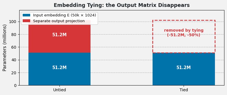
    Bar chart comparing parameter counts of untied versus tied configurations, showing the output projection matrix of fifty million parameters eliminated by tying.

    Figure 2: Tying deletes the output projection matrix, one of the largest single blocks of parameters in vocabulary-heavy models.

    Vocabulary Mismatch Caveat: Tying assumes input and output share a vocabulary. When source and target vocabularies differ (multilingual translation), only the decoder input embedding and output projection can be tied; the encoder embedding stays separate.


    Login to view more content
  • DL0038 Transformer Activation

    Which activation functions do transformer models use?

    Answer

    Transformers use activations in two places. Inside the FFN, the hidden layer applies ReLU (original paper) or, in most modern models, GELU. BERT, GPT, and ViT all standardized on GELU, and newer LLMs adopt gated variants like SwiGLU. Inside attention, softmax normalizes the score matrix into attention weights. The GELU/ReLU choice controls gradient health; softmax controls score interpretability.

    (1) GELU (FFN, modern default): Smooth, probabilistic gating: small negative inputs survive with tiny gradients, avoiding dead neurons and smoothing optimization.
    (2) ReLU (FFN, original): \max(0, x), cheap and effective, but its hard zero can kill neurons permanently.
    (3) Softmax (attention): Converts raw scores into a normalized distribution over keys, giving every query a convex combination of value vectors.

    Single plot comparing ReLU, GELU, and SiLU curves from minus three to three, with ReLU clamping all negatives to zero while GELU and SiLU smoothly dip below zero before rising.

    Figure 1: ReLU clamps negatives to a hard zero; GELU curves smoothly through them: small negative activations keep a non-zero gradient.

    Mathematical Formulation:
    \mathrm{GELU}(x) = x \cdot \Phi(x) = x \cdot \frac{1}{2}\left[1 + \mathrm{erf}\left(\frac{x}{\sqrt{2}}\right)\right]
    \mathrm{Softmax}(z_i) = \frac{e^{z_i}}{\sum_{j=1}^{K} e^{z_j}}

    Where:

    • \Phi(x) is the standard Gaussian CDF: GELU gates the input by its own probability of being positive, a smooth stochastic-regularization view.
    • z_i is one raw attention score and K the number of scored keys; softmax outputs sum to 1.

    Why GELU Won: Its smoothness yields non-zero gradients for negative inputs, reducing the “Dying ReLU” failure; the data-dependent gating acts like a soft, learned threshold. Empirically this means more stable training and better final loss in large language and vision models, which is why BERT/GPT-era models abandoned ReLU in the FFN.

    Flowchart of one Transformer block marking the two activation sites: softmax inside scaled dot-product attention after the score matrix, and GELU between the two linear layers of the feed-forward network.

    Figure 2: The two activation sites in every block: softmax in attention, GELU/ReLU between the FFN’s two linear layers.

    Beyond GELU: Recent LLMs (PaLM, LLaMA) replace the plain activation with gated linear units (SwiGLU/GEGLU), where one projection’s activation multiplies another linear path elementwise; this gating adds quality per parameter and has become the default in state-of-the-art FFN design.


    Login to view more content
  • DL0037 Transformer Architecture III

    Why do Transformers use a dot product, rather than addition, to compute attention scores?

    Answer

    The dot product is a natural similarity measure: q \cdot k is large exactly when query and key point in the same direction, so it directly expresses “how relevant is this key to my query”. It is also a single fused matrix multiplication (QK^\top scores all pairs at once), which is far faster on modern hardware than additive attention’s per-pair MLP. Scaling by 1/\sqrt{d_k} keeps it numerically stable in high dimensions.

    (1) Geometric Meaning: q \cdot k = \|q\|\,\|k\|\cos\theta: aligned vectors score high, orthogonal vectors score zero, opposed vectors score negative.
    (2) Hardware Efficiency: All scores materialize as one GEMM QK^\top; additive attention needs an MLP evaluated for every (query, key) pair.
    (3) Probabilistic Readout: Softmax over dot-product scores yields interpretable attention weights: a distribution over which keys matter.

    2D vector diagram showing three vectors from the origin with a positive dot product between two aligned vectors and a negative dot product between two opposed vectors.

    Figure 1: Dot product as similarity: aligned vectors score positive, opposed vectors score negative; softmax turns scores into attention weights.

    Mathematical Formulation:
    \alpha_i = \frac{e^{q \cdot k_i / \sqrt{d_k}}}{\sum_{j=1}^{n} e^{q \cdot k_j / \sqrt{d_k}}}

    Where:

    • \alpha_i is the attention weight the query assigns to key k_i; weights sum to 1 over the n keys.
    • q \cdot k_i is the dot-product similarity; \sqrt{d_k} scaling prevents softmax saturation for large key dimension d_k.

    Why Not Addition: Adding features component-wise, q + k, says nothing about alignment; two very different pairs can sum to the same vector. To become a usable score, the sum must pass through an extra learnable MLP (v^\top \tanh(W_q q + W_k k)), which is slower per pair and still lacks the dot product’s direct geometric interpretation.

    Comparison flowchart of dot-product attention scoring all pairs in one matrix multiply versus additive attention pushing each query-key pair through a small neural network scorer.

    Figure 2: Dot-product scoring = one batched GEMM; additive scoring = a per-pair MLP, richer but much slower at scale.

    The One Caveat: For large d_k, raw dot products grow in variance proportional to d_k, pushing softmax into saturated, gradient-poor regions, which is why the Transformer uses the scaled dot product rather than the plain one.


    Login to view more content