Explain “Positional Encoding” in Transformers. Why is it necessary?
Answer
Positional encoding is crucial in Transformers to equip the model with an understanding of token order while maintaining full parallel computation. Fixed sinusoidal functions offer parameter-free generalization to unseen lengths, learned embeddings provide task-specific flexibility, and relative schemes directly capture inter-token distances.
Self-attention is permutation-invariant and, on its own, cannot distinguish token order. Positional encodings inject sequence information by adding position-dependent vectors to token embeddings.
Encoding types:
(1) Fixed (sinusoidal): Predefined functions of position. Sinusoidal (fixed) encodings utilize sine and cosine functions at different frequencies, enabling the model to learn both relative and absolute positions.
(2) Learned: Learned during training as parameters. Learned positional embeddings are trainable vectors but may not generalize beyond the maximum training length.
Sinusoidal Encoding Formula:

Where: : token position in the sequence
 : dimension index
 : embedding dimension
The figure below shows how the encoding values change across different positions and dimensions.
 to a lower bound depending on the sparsity pattern.
 is computed only at dilated positions:
 are the dilated subsets of keys and values.
 is the key dimension.
 (e.g., the token itself and
  neighbors).
 .
.


 : Final output projection matrix that maps the concatenated attention outputs back to the original model dimension.
 : Number of attention heads.
 : Dimension of each head’s projected subspace.
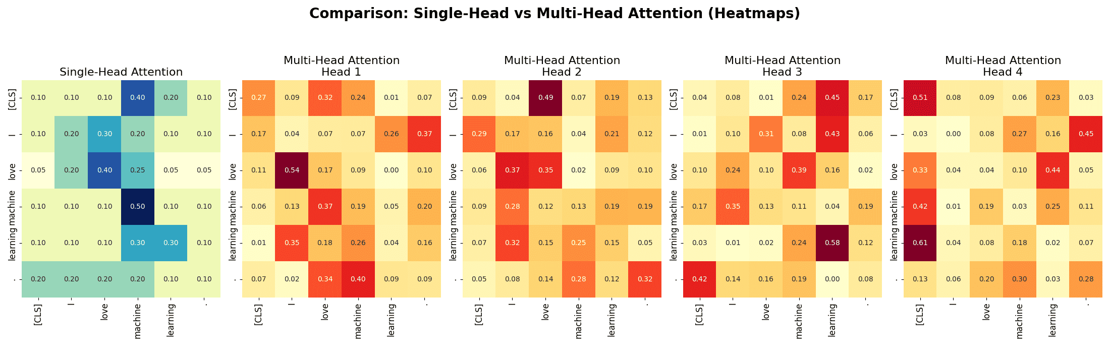

 ,
,  , and
, and  represent query, key, and value matrices, respectively
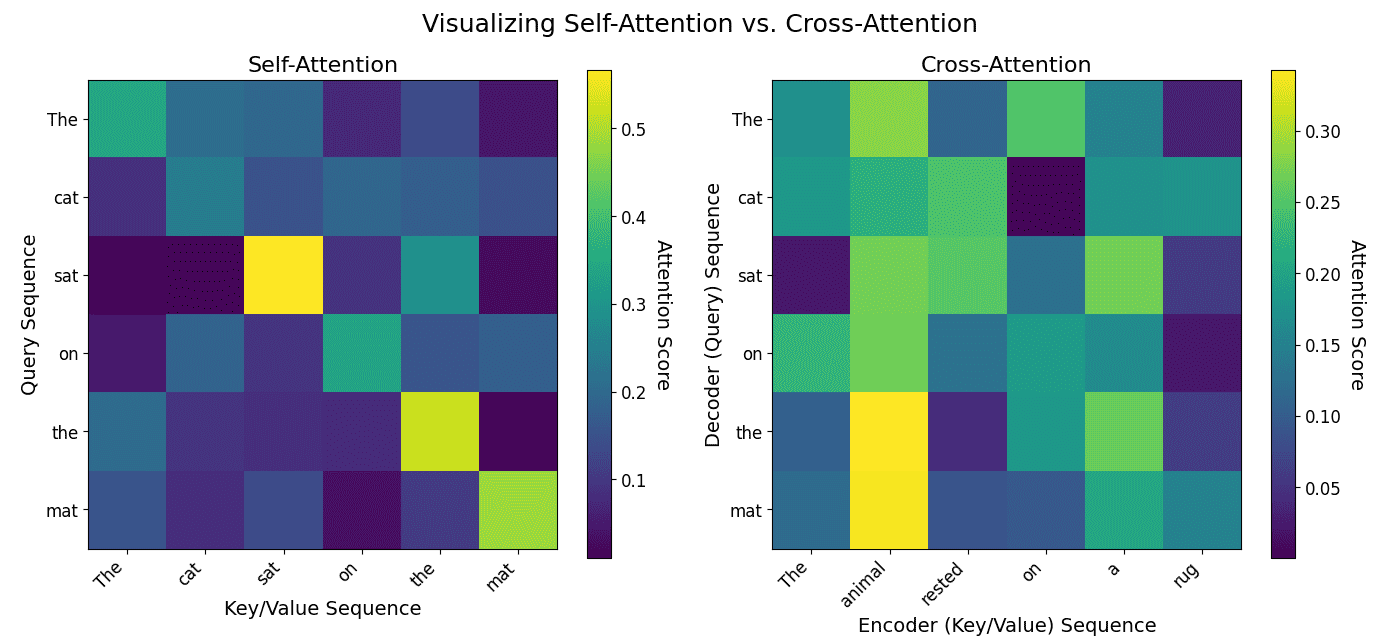

 : Matrices of queries, keys, and values.
 : Converts similarity scores to probabilities.
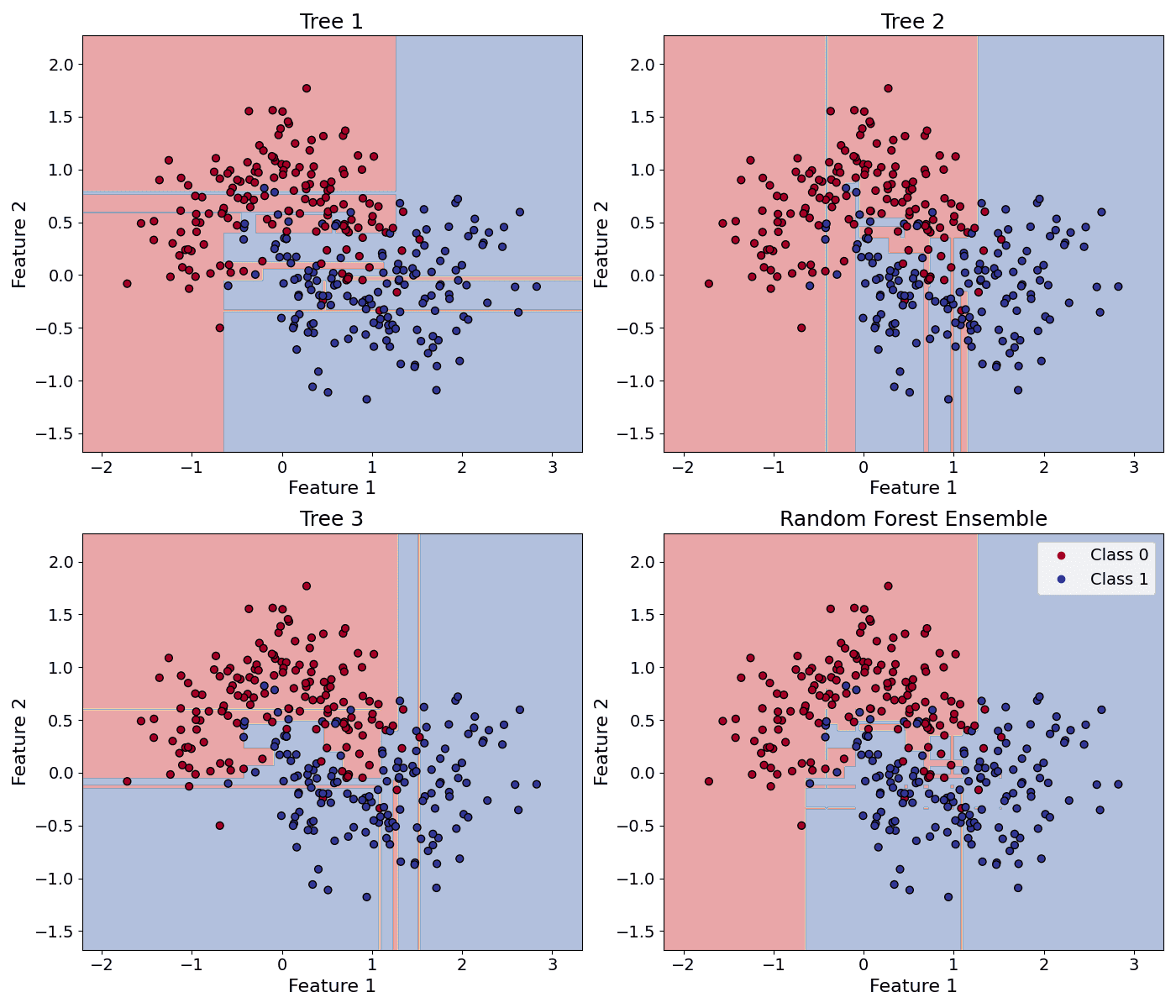
 ) using rules of thumb (default heuristics), then tune via cross-validation or out-of-bag (OOB) error to find the best value for your specific dataset.

 = total number of features,
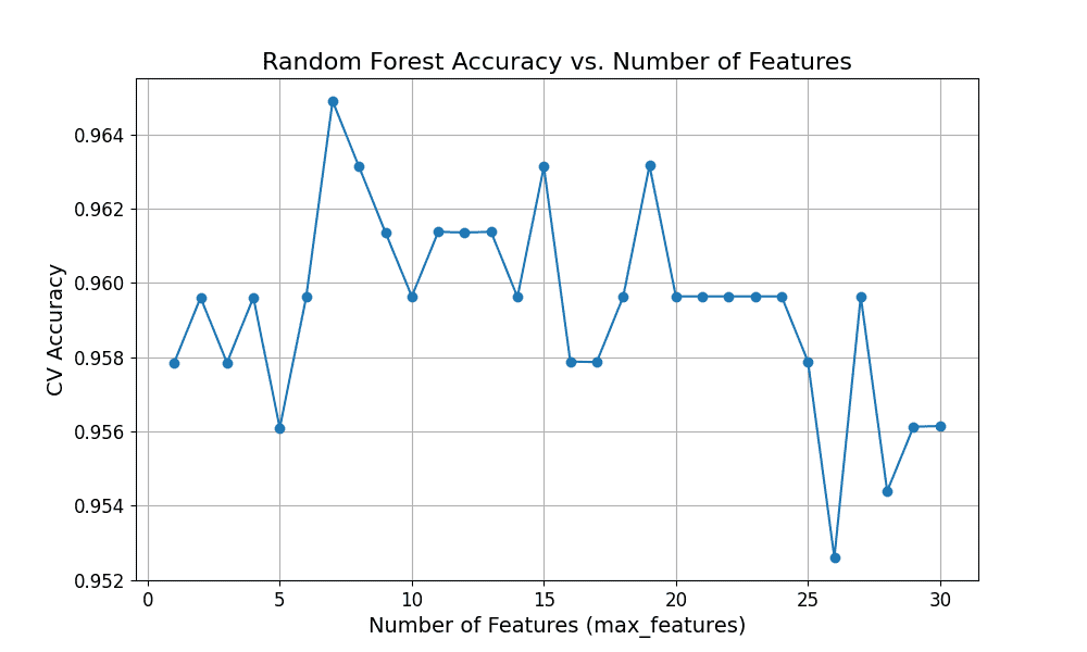

 = prediction of the b-th tree.
 = total number of trees.