Describe the original Transformer encoder–decoder architecture.
Answer
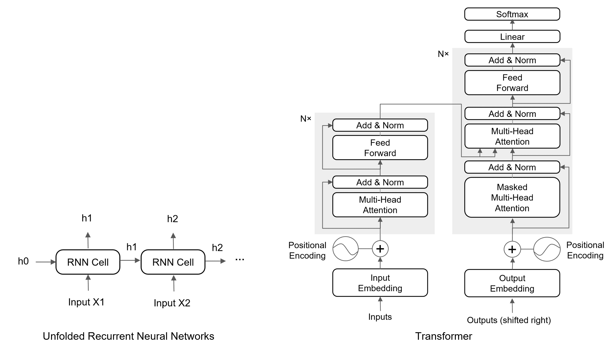
The original Transformer model has an encoder-decoder architecture. The encoder processes the input sequence (e.g., a sentence) to create a contextual representation for each word. The decoder then uses this representation to generate the output sequence (e.g., the translated sentence), one word at a time. This entire process relies on attention mechanisms instead of recurrence.
Overall: Sequence-to-sequence encoder–decoder model with 6 encoder layers and 6 decoder layers [1].
Encoder layer:
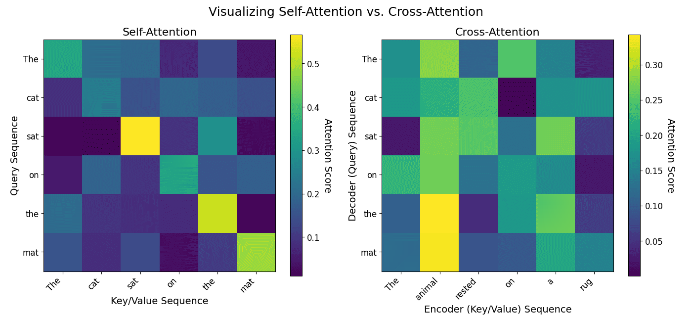
(1) Multi-Head Self-Attention (all tokens attend to each other).
(2) Position-wise Feed-Forward Network (two linear layers + ReLU).
(3) Residual connection + LayerNorm after each sublayer.
Decoder layer:
(1) Masked Multi-Head Self-Attention (prevents seeing future tokens).
(2) Cross-Attention (queries from decoder, keys/values from encoder output).
(3) Position-wise Feed-Forward Network.
(4) Residual connection + LayerNorm after each sublayer.
Input representation: Inputs are represented as token embeddings summed with positional encodings to preserve sequence order, as the attention mechanism is permutation-invariant.
Output: The final decoder output passes through a linear projection layer, followed by softmax to produce probabilities over the target vocabulary for next-token prediction.
The figure below shows the architecture of the Transformer.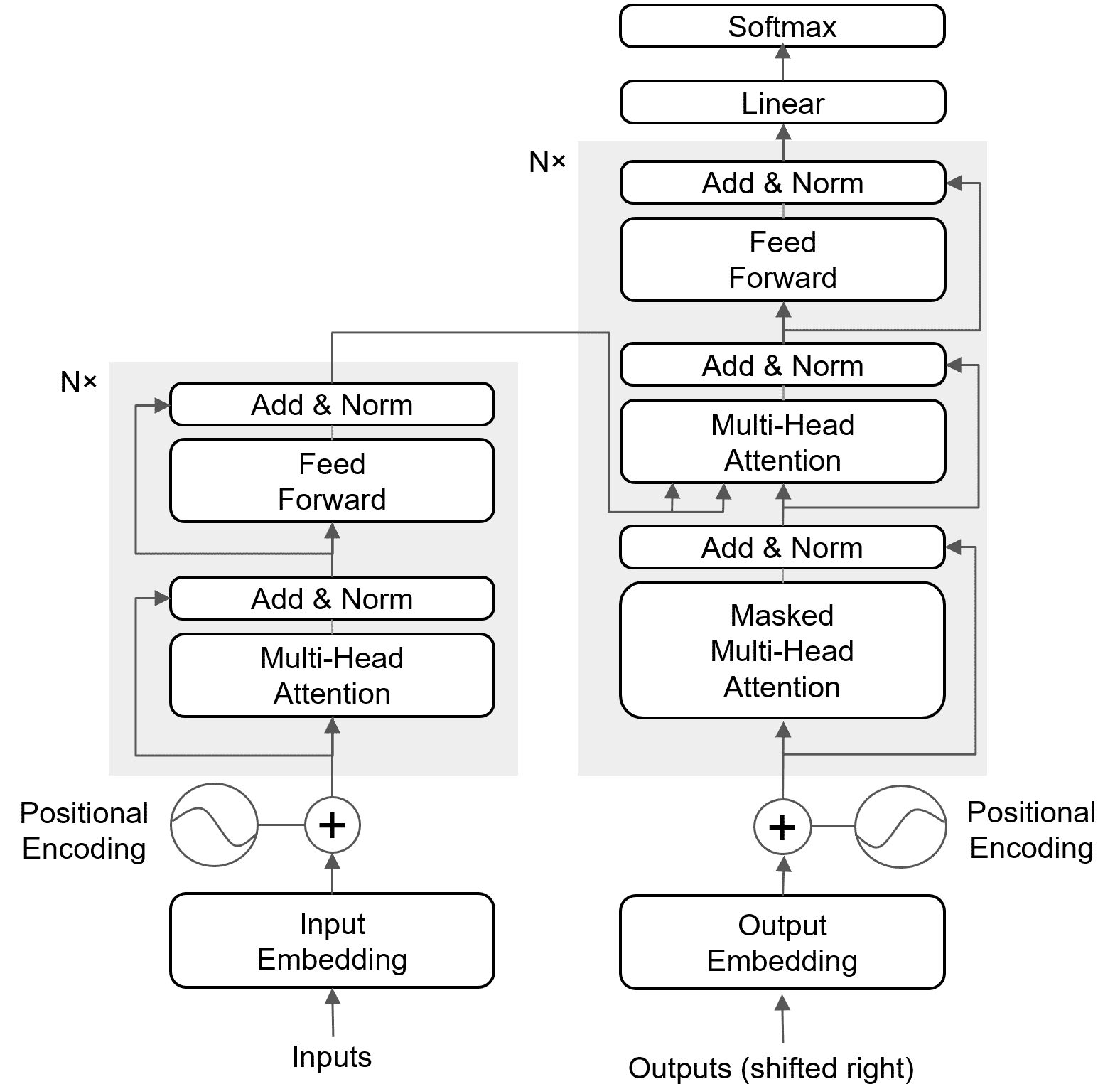
References:
[1] Vaswani, Ashish, et al. “Attention is all you need.” Advances in neural information processing systems 30 (2017).

 = input feature,
 = mean of all features for the current sample,
 = standard deviation of all features,
 = small constant for numerical stability,
 = learnable scale and shift parameters.
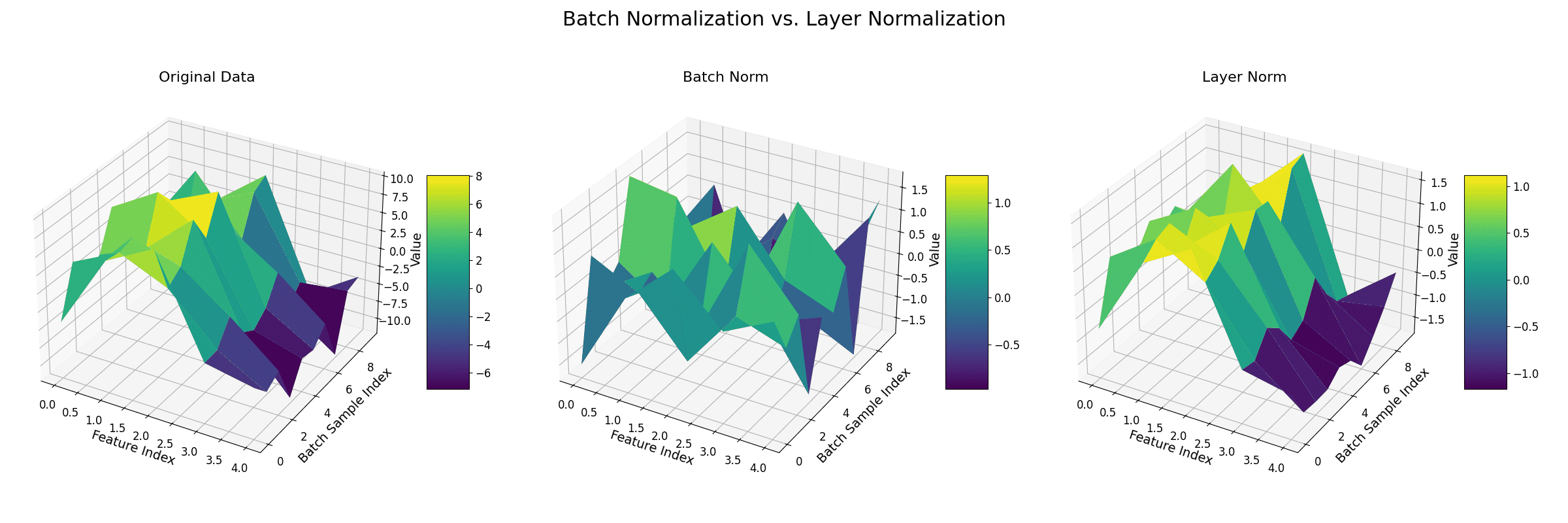
 ): Cost is relatively small; attention score matrix overhead is minimal. Q, K, and V projections together dominate the compute.

 is large.
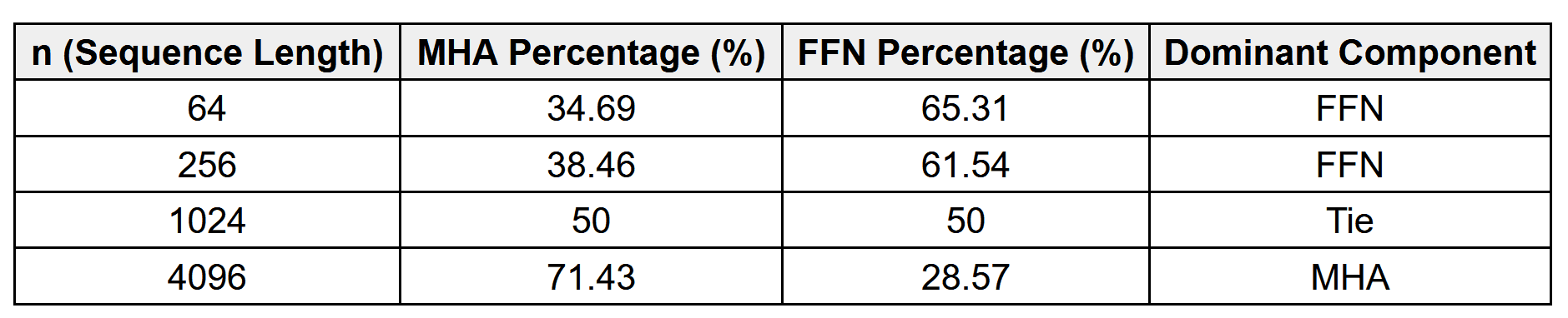

 — input vector for a token after the attention layer
 — trainable weight matrices
 — trainable bias vectors
 — ReLU activation (sometimes replaced by GELU)

 : token position in the sequence
 : dimension index
 : embedding dimension
 to a lower bound depending on the sparsity pattern.
 is computed only at dilated positions:
 are the dilated subsets of keys and values.
 is the key dimension.
 (e.g., the token itself and
  neighbors).
 .
.


 : Final output projection matrix that maps the concatenated attention outputs back to the original model dimension.
 : Number of attention heads.
 : Dimension of each head’s projected subspace.

 ,
,  , and
, and  represent query, key, and value matrices, respectively