Author: admin

  • ML0063 Random Forest

    How does the random forest algorithm operate? Please outline its key steps.

    Answer

    Random Forest builds an ensemble of decision trees, each trained on a bootstrapped sample of the data with a random feature subset considered at each split. This combination reduces variance, combats overfitting, and improves predictive accuracy; the final output aggregates all trees’ predictions: majority vote for classification, averaging for regression.

    (1) Bootstrap Sampling: Create multiple subsets of the training data by sampling with replacement (bootstrap samples).
    (2) Grow Decision Trees: Train an unpruned decision tree on each bootstrap sample.
    (3) Random Feature Selection: At every split in every tree, consider only a random subset of features; this increases diversity between trees.
    (4) Aggregate: Classification: each tree votes for a class and the majority wins; regression: the tree outputs are averaged.

    Three individual tree decision boundaries with different jagged artifacts and the smoother random forest ensemble boundary

    Figure 1: Three trees, three different jagged boundaries: each overfits its own bootstrap sample in its own way. The ensemble’s boundary (bottom right) averages the votes and lands smoother and closer to the true structure: the trees’ individual errors cancel.

    Mathematical Formulation:
    \hat{y} = \mathrm{mode}\big\{ T_b(x) \big\},\quad b = 1, \ldots, B
    \hat{y} = \frac{1}{B} \sum_{b=1}^{B} T_b(x)

    Where:

    • T_b(x) is the prediction of the b-th tree for input x.
    • B is the total number of trees in the forest.
    • First line: classification by majority vote (mode); second line: regression by averaging.
    Flowchart from training data through bootstrap samples into three trees and a majority vote box producing the final prediction

    Figure 2: The full pipeline: B bootstrap replicas of the training set feed B independently grown trees (each with random feature subsets at its splits), and a majority-vote / averaging box fuses their outputs into one robust prediction.


    Login to view more content
  • ML0062 Decision Tree

    Please explain how a decision tree works.

    Answer

    A decision tree partitions the input space into regions by recursively splitting on the feature that best separates the target variable. Each split aims to improve the “purity” of the resulting subsets, measured by criteria such as Gini impurity or entropy. Predictions follow the sequence of splits down to a leaf, returning the most common class (classification) or the average target (regression).

    (1) Structure: A tree of nodes: internal nodes test a feature, branches represent the outcomes, leaves give predictions.
    (2) Splitting Criterion: Choose the best feature and threshold by maximizing purity: information gain (entropy), Gini impurity, or variance reduction for regression.
    (3) Recursive Growth: Starting at the root, split the data, then recurse on each subset until stopping criteria are met (max depth, min samples, or pure leaves).
    (4) Prediction: A new sample travels from root to leaf following the feature tests; the leaf’s label or value is returned.

    Left panel 2-D data partitioned by axis aligned decision regions, right panel the corresponding tree with gini and sample counts at each node

    Figure 1: A decision tree from two viewpoints: on the left, the axis-aligned rectangular regions it carves into the feature space; on the right, the tree itself: each node shows its test, impurity, and class counts, and each leaf is a final answer.

    Mathematical Formulation:
    \mathrm{Gini}(t) = 1 - \sum_{k=1}^{K} p_k^2
    \mathrm{Entropy}(t) = -\sum_{k=1}^{K} p_k \log_2(p_k)
    \mathrm{Information\ Gain} = \mathrm{Entropy}(\mathrm{Parent}) - \sum_{i} \frac{N_i}{N} \, \mathrm{Entropy}(\mathrm{Child}_i)

    Where:

    • t is a tree node; K the number of classes; p_k the proportion of class k samples in node t.
    • Gini = 0 means the node is pure (one class only) and grows with mixing; entropy = 0 at perfect purity and is maximal when classes are uniformly mixed.
    • In the gain formula, N is the parent’s sample count and N_i child i‘s: the split chosen is the one maximizing this weighted impurity drop.
    Gini and entropy impurity curves versus class probability both peaking at one half and zero at the extremes

    Figure 2: The two classification criteria compared for a binary node: both peak at p = 0.5 (maximally mixed) and vanish at pure nodes; they nearly always rank candidate splits in the same order, which is why Gini (no logarithms) is the common default.


    Login to view more content
  • ML0061 KNN and K-means

    What are the key differences between KNN and K-means?

    Answer

    KNN (K-Nearest Neighbors) is a supervised algorithm that classifies data using the labels of its nearest neighbors: prediction from historical labeled data. K-means is an unsupervised clustering technique that groups data purely by similarity, using no labels at all. Despite the shared “K”, they solve different problems.

    (1) Learning Type: KNN is supervised (classification/regression); K-means is unsupervised (clustering).
    (2) Objective: KNN predicts a new sample’s label from the majority vote (or average) of its K nearest neighbors; K-means partitions the dataset into K clusters by minimizing intra-cluster distance.
    (3) Training: KNN has no explicit training: it stores the entire dataset; K-means iteratively learns cluster centroids.
    (4) Prediction Cost: KNN is expensive at prediction (distance to every training point, sort, take the top K, then vote/average); K-means is cheap: distances to K centroids, assign the nearest.
    (5) Distance Use And Output: KNN uses distance to find neighbors and outputs a label or value; K-means uses distance to assign points to centroids and outputs cluster assignments plus centroids.

    FeatureK-Nearest Neighbors (KNN)K-Means
    TypeSupervised LearningUnsupervised Learning
    TaskClassification, RegressionClustering
    Data RequiredLabeled dataUnlabeled data
    Training PhaseStores all training data (lazy learner)Iterative centroid calculation
    Prediction PhaseFinds K nearest neighbors and assigns label/valueAssigns new points to closest cluster centroid
    Compute CostHigh at prediction (distance calculations for each new point)High at training (iterative updates); low at prediction (centroid assignment)
    GoalPredict label/value for new dataGroup data into K clusters
    OutputClass label or predicted valueData points assigned to clusters

    Mathematical Formulation:
    \hat{y} = \arg\max_{c \in \mathcal{C}} \; \sum_{i=1}^{K} \mathbb{1}(y_i = c)
    \min_{C_1, \ldots, C_K} \; \sum_{k=1}^{K} \sum_{x \in C_k} \|x - \mu_k\|^2

    Where:

    • KNN (first line): \hat{y} is the predicted class, \mathcal{C} the class set, y_i the label of the i-th nearest neighbor, and \mathbb{1}(\cdot) the vote-counting indicator.
    • K-means (second line): C_k is cluster k and \mu_k its centroid; the algorithm minimizes total within-cluster squared distance: no labels appear anywhere.
    Two panels on crescent moon data showing KNN separating the moons correctly while K-means cuts through them

    Figure 1: Same data, different goals: with labels, KNN’s local votes trace the two crescents perfectly (left); without labels, K-means can only split by nearest-centroid geometry and slices through both moons (right). KNN performs well here thanks to local decision-making; K-means fails because it assumes spherical clusters with linear boundaries.


    Login to view more content
  • ML0060 K Selection in K-Means

    How to select K in K-Means?

    Answer

    To select the optimal number of clusters K in K-means, combine visual tools (the elbow method), quantitative metrics (the silhouette score), and statistical methods (the gap statistic), balancing model fit against generalization without overfitting. Domain knowledge and interpretability should have the final word.

    (1) Elbow Method: Plot within-cluster sum of squares (WCSS) against K and pick the “elbow” where the rate of improvement sharply slows.
    (2) Silhouette Score: Compute the average silhouette coefficient for each candidate K and pick the highest: it rewards tight, well-separated clusters.
    (3) Gap Statistic: Compare the observed WCSS against that of a random reference distribution; pick the K maximizing the gap.

    WCSS curve dropping steeply from K equals 1 and flattening after the marked elbow at K equals 3

    Figure 1: The elbow method: WCSS always decreases as K grows, but the marginal gain collapses after the true cluster count (the marked elbow at K = 3). Beyond the elbow you pay model complexity for noise.

    Mathematical Formulation:
    \text{WCSS}(K) = \sum_{k=1}^{K} \sum_{x_i \in C_k} \|x_i - \mu_k\|^2
    s(i) = \frac{b(i) - a(i)}{\max\big(a(i),\, b(i)\big)}

    Where:

    • C_k is cluster k and \mu_k its centroid; WCSS is the total within-cluster squared distance that the elbow method plots against K.
    • a(i) is point i‘s mean distance to its own cluster (intra-cluster); b(i) its mean distance to the nearest other cluster.
    • s(i) \in [-1, 1]: near 1 means well clustered, near 0 means on a boundary, negative means likely misassigned; average it over all points for each K.

    Login to view more content
  • ML0059 K-means II

    K-Means is widely used for clustering. Can you discuss its main benefits as well as its disadvantages?

    Answer

    K-means partitions data into K clusters where each point belongs to the cluster with the nearest mean. It is computationally efficient and easy to implement, but it requires specifying the number of clusters in advance, assumes spherical clusters, and is sensitive to initialization and outliers.

    (1) Simple And Efficient: Fast to compute, easy to implement, and scalable to large datasets.
    (2) Unsupervised And Interpretable: Needs no labels, and the centroids are intuitive summaries of each cluster.
    (3) Strong Assumptions: Works best on compact, well-separated spherical clusters; the user must fix K beforehand.
    (4) Fragility: Poor initial centroids can lock in suboptimal results, outliers drag centroids, and plain Euclidean distance excludes non-numeric features.

    Mathematical Formulation:
    J = \sum_{i=1}^{K} \sum_{x_j \in C_i} \|x_j - \mu_i\|^2

    Where:

    • K is the number of clusters; C_i the set of points in cluster i.
    • \mu_i is the centroid of cluster i; x_j a data point assigned to it.
    • J is the within-cluster sum of squared distances: the objective both steps of the algorithm drive down monotonically.
    Left panel K-means succeeding on three spherical clusters, right panel K-means cutting through two crescent shaped clusters

    Figure 1: The assumption made visible: on spherical, well-separated blobs (left) K-means nails the structure; on two crescents (right) its linear, centroid-based split slices through both moons: the spherical-cluster assumption failing in action.


    Login to view more content
  • ML0058 K-means++

    Please explain how K-means++ works.

    Answer

    K-means++ is an improved way to initialize the centroids of K-means. Instead of picking all centroids uniformly at random, it selects them one by one with probability proportional to the squared distance from the already chosen centroids. This spreads the initial centroids out, sharply reducing the chance of poor clustering and helping the algorithm converge faster and more reliably. After initialization, standard K-means proceeds unchanged.

    (1) First Centroid: Choose \mu_1 uniformly at random from the dataset.
    (2) Distance Computation: For each point, compute its squared distance to the nearest already-chosen centroid.
    (3) Weighted Selection: Pick the next centroid with probability proportional to that squared distance: far points are favored.
    (4) Repeat Until K: Continue until all K centroids are chosen, then run standard K-means.

    Five clusters with centroids initialized by K-means plus plus landing one per cluster

    Figure 1: K-means++ initialization (K=5): the distance-squared weighting spreads the starting centroids across all five natural groups, so the algorithm starts close to a good solution instead of gambling on random seeds.

    Mathematical Formulation:
    D(x_i)^2 = \min_{1 \le j \le m} \|x_i - \mu_j\|^2
    P(x_i) = \frac{D(x_i)^2}{\sum_j D(x_j)^2}

    Where:

    • \mu_j is one of the m already chosen centroids; D(x_i)^2 is point x_i‘s squared distance to its nearest chosen centroid.
    • P(x_i) is the probability of x_i becoming the next centroid, proportional to D(x_i)^2, so points far from every chosen centroid are exponentially favored over nearby ones.
    • The denominator normalizes over all data points; selection repeats until K centroids exist.
    Side by side comparison where random initialization merges two groups and splits one while K-means plus plus finds all three true clusters

    Figure 2: Why initialization matters: with an unlucky random init (left), two centroids land in one group and the small top cluster is merged away; K-means++ (right) seeds one centroid per group and recovers all three clusters cleanly.


    Login to view more content
  • ML0057 K-means

    Please explain how K-means works.

    Answer

    K-means is an iterative unsupervised algorithm that partitions data into K clusters by minimizing intra-cluster distances (within-cluster variance). It alternates between assigning points to the nearest centroid and recomputing centroids until convergence. It is fast and easy to implement, but sensitive to initialization and to non-convex cluster shapes.

    (1) Initialization: Choose K initial centroids (randomly, or with K-means++).
    (2) Assignment Step: Assign every point to its closest centroid by Euclidean distance.
    (3) Update Step: Recompute each centroid as the mean of the points assigned to it.
    (4) Convergence: Repeat assignment and update until the centroids stabilize or a stopping criterion is met.

    Three well separated clusters colored by assignment with red X markers at the learned centroids

    Figure 1: K-means (K=3) converged on blob data: colors mark the final assignments and the red X’s are the centroids: each is the mean of its cluster, and every point belongs to its nearest centroid’s cluster.

    Mathematical Formulation:
    d(x, c_k) = \sqrt{\sum_{i=1}^{n} (x_i - c_{k,i})^2}
    c_k = \frac{1}{|C_k|} \sum_{x \in C_k} x

    Where:

    • x is a data point and c_k the centroid of cluster k (first formula: Euclidean assignment distance, n = number of features).
    • C_k is the set of points currently assigned to cluster k; the update sets the centroid to their component-wise mean, the minimizer of squared distances for a fixed assignment.

    Login to view more content
  • ML0056 K Selection in KNN

    In the context of designing a K-Nearest Neighbors (KNN) model, can you explain your approach to selecting the value of K?

    Answer

    Selecting K in KNN is crucial because it directly controls model performance through the bias-variance tradeoff. The systematic approach is k-fold cross-validation combined with grid search over a range of K values, picking the one that minimizes validation error, informed where possible by domain knowledge and data characteristics.

    (1) Bias-Variance Tradeoff: A small K (e.g., 1) gives low bias but high variance: it tracks noise and overfits; a large K raises bias but lowers variance: it oversmooths and can underfit.
    (2) Use Odd Values For Classification: In binary classification, an odd K avoids tie votes.
    (3) Cross-Validation + Grid Search: Evaluate every candidate K with k-fold CV and select the minimizer of validation error.
    (4) Domain Knowledge: Prior knowledge of the data distribution can narrow the search range.

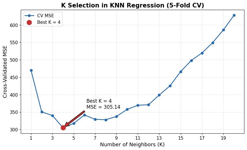
    Cross validated MSE curve over K from 1 to 20 with a minimum marked at K equals 4

    Figure 1: 5-fold CV error across K on a regression task: error dives as variance is tamed (tiny K overfits), bottoms at K = 4, then climbs steadily as over-averaging sets in (large K underfits). The minimizer is the selected K.

    Mathematical Formulation:
    CV(K) = \frac{1}{N} \sum_{i=1}^{N} \ell\big(y_i, \hat{y}_i(K)\big)

    Where:

    • y_i is the actual outcome for the i-th validation instance.
    • \hat{y}_i(K) is the prediction made using K neighbors (with the point’s own fold held out).
    • N is the number of validation samples and \ell the loss (e.g., squared error for regression, 0-1 for classification).

    Login to view more content
  • ML0055 KNN Regression

    Please explain how KNN Regression works.

    Answer

    K-Nearest Neighbors (KNN) Regression is a simple, instance-based algorithm that predicts a continuous output by finding the K nearest training points and averaging their target values. Its simplicity makes it easy to understand and implement, but performance is sensitive to K and the distance metric, and prediction is computationally expensive on large datasets since every query compares against all training samples. Like its classification sibling, KNN regression is a “lazy learner”: it builds no explicit model and simply memorizes the training data.

    (1) Instance-Based: No explicit model is learned; predictions come from stored training data and similarity.
    (2) Distance-Based: Find the K nearest neighbors of the query point (commonly Euclidean distance).
    (3) Averaging Neighbors: The prediction is the mean of those neighbors’ target values.
    (4) Sensitive To K And Metric: Small K tracks noise; large K oversmooths.
    (5) No Training Phase: All computation happens during prediction.

    KNN regression with K equals five predicting a jagged step like curve through noisy sinusoidal training points

    Figure 1: KNN regression (K=5) on a noisy sine wave: each prediction averages the 5 nearest targets, producing a locally-flat, step-like curve that follows the trend but clips the peaks and troughs, the signature of local averaging.

    Mathematical Formulation:
    \hat{y} = \frac{1}{K} \sum_{i=1}^{K} y_i
    \hat{y}(x_q) = \frac{\sum_{i=1}^{K} w_i \cdot y_i}{\sum_{i=1}^{K} w_i}
    w_i = \frac{1}{d(x_q, x_i) + \epsilon}

    Where:

    • \hat{y} is the prediction for the query point; y_i the target of the i-th nearest neighbor; K the number of neighbors (first formula: uniform average).
    • In the weighted variant, w_i is inversely proportional to the distance d(x_q, x_i) between query and neighbor: closer points influence the prediction more.
    • \epsilon is a small constant avoiding division by zero when a neighbor sits exactly on the query.

    Login to view more content
  • ML0054 KNN Classification

    Please explain how KNN classification works.

    Answer

    K-Nearest Neighbors (KNN) is a simple, non-parametric algorithm that predicts a label by majority vote among the K nearest neighbors of a test point, using a chosen distance metric. It is intuitive and effective for small datasets, though less efficient on large-scale data.

    (1) Instance-Based Method: KNN learns no explicit model; it stores the training data and predicts from similarity.
    (2) Distance-Based Classification: For a test point, it computes the distance to every training point (e.g., Euclidean).
    (3) Majority Vote: It selects the K closest neighbors and assigns the most frequent label among them.
    (4) Sensitive To K And Metric: Performance depends on the choice of K and the distance measure (Euclidean, Manhattan, …).
    (5) No Training Phase: All computation happens at prediction time: hence “lazy learning”.

    KNN with K equals five decision regions over two classes where only the horizontal feature is informative

    Figure 1: KNN (K=5) decision regions: the boundary wiggles because each query point polls its 5 nearest neighbors: local votes trace the class structure instead of fitting a global line. Note only Feature 1 is informative here; the vertical wiggle is the noise feature leaking into the vote.

    Mathematical Formulation:
    \mathrm{distance}(x, y) = \sqrt{\sum_{i=1}^{n} (x_i - y_i)^2}
    \hat{y} = \arg\max_{c \in \mathcal{C}} \; \sum_{i=1}^{K} \mathbb{1}(y_i = c)

    Where:

    • x_i and y_i are the i-th features of the query and training points; n is the number of features (first formula: Euclidean distance).
    • \hat{y} is the predicted class for the query point; \mathcal{C} is the set of all classes; K is the number of neighbors polled.
    • y_i is the label of the i-th neighbor and \mathbb{1}(y_i = c) the indicator counting that neighbor’s vote for class c.

    Login to view more content